Collective motion is one of the most spectacular manifestations of coordinated behavior in nature. From bird flocks to fish schools, insect swarms to bacterial colonies, the synchronized movement of multiple individuals without centralized control is a ubiquitous phenomenon across biological scales.
Biological swarms represent natural examples of self-organized collective behavior that has evolved over millions of years. They demonstrate how simple local interaction rules can give rise to complex global patterns, making them perfect examples of emergent phenomena.
The study of biological swarms offers multiple benefits:
It deepens our understanding of fundamental biological processes
It provides inspiration for engineered systems like robot swarms
It offers insights applicable to diverse fields including traffic management, crowd control, and network theory
Bird Flocks: Starling Murmurations
Starling murmurations represent one of nature’s most breathtaking displays of collective behavior. These aerial performances, involving thousands to hundreds of thousands of birds, showcase remarkable coordination as the flock changes shape, splits, and merges while maintaining cohesion.
The spectacular patterns formed by starling flocks are particularly visible at dusk when large numbers gather before roosting. The rapid changes in direction propagate across the flock in wave-like patterns that seem to flow like a liquid, creating mesmerizing, ever-changing shapes against the sky.
For excellent visual representations of starling murmurations, see the work of Cavagna et al. (2010), which presents time-lapse photography of murmurations with velocity field overlays, demonstrating the coordination of movement across thousands of individuals.
The STARFLAG (Starlings in Flight) project, led by researchers including Cavagna, Giardina, and others, revolutionized our understanding of bird flocks through rigorous quantitative analysis. Using multiple high-speed cameras calibrated to reconstruct three-dimensional positions of individual birds within flocks of thousands, they made several groundbreaking discoveries:
The team found that correlations in velocity fluctuations extend throughout the entire flock, regardless of its size—a phenomenon called scale-free correlations. This finding, detailed in Cavagna et al. (2010, PNAS), suggests that flocks behave as critical systems poised at a phase transition, allowing information to propagate rapidly throughout the group. Their research demonstrates correlation functions that exhibit this scale-free property.
Another key discovery was that birds interact based on topological rather than metric distance. Each bird coordinates with a fixed number of neighbors (typically 6-7) regardless of their physical distance, rather than with all neighbors within a certain radius. This finding, published in Ballerini et al. (2008, PNAS), explains how flocks maintain cohesion even when changing density during maneuvers. Their study clearly illustrates this topological interaction network.
Information transfer within flocks occurs remarkably fast, with directional changes propagating across hundreds of meters in less than a second. This allows starlings to respond collectively to predator attacks with near-instantaneous coordination. Attanasi et al. (2014, Nature Physics) documented this phenomenon, showing in their analysis how information waves propagate through the flock at speeds faster than what would be predicted by nearest-neighbor interactions alone.
When comparing starling flocks to the Vicsek model, we find significant similarities in the basic alignment mechanism—both real birds and simulated particles tend to align their direction of motion with neighbors. However, real starlings use topological rather than metric interactions, a critical difference that affects how the system behaves, particularly during density changes.
Bialek et al. (2012, PNAS) showed that the directional correlation functions observed in real flocks resemble those found in critical systems, suggesting that flocks operate near phase transitions that maximize their response to external perturbations like predator attacks. Their results illustrate how the maximum entropy model derived from real flock data exhibits critical behavior.
Models incorporating topological interactions show much better agreement with empirical data. Ginelli and Chaté (2010, Physical Review Letters) demonstrated that topological Vicsek-type models reproduce the scale-free correlations observed in real flocks, as shown in their research, which directly compares correlation lengths in metric versus topological models.
The information propagation observed in starling flocks is wave-like, similar to the predictions from Toner-Tu theory. Attanasi et al. (2014) measured the speed of information transfer through flocks during turning events, finding propagation speeds consistent with the sound-like modes predicted by the hydrodynamic theory.
Quantitative Analysis of Collective Motion
The Vicsek model and its flocking transition were introduced in Lecture 7. Here we use it as a quantitative tool, focusing on the order parameters and correlation functions that connect the model to measurements on real animal groups.
Order Parameters and Correlation Functions
To quantitatively characterize collective motion, we need mathematical measures that capture the degree of organization in a system. The most fundamental measure is the polarization order parameter, defined as:
where \(\mathbf{v}_i\) is the velocity of particle \(i\) and \(N\) is the total number of particles. This parameter ranges from \(\Phi = 0\) (completely disordered, random directions) to \(\Phi = 1\) (perfectly aligned, all particles moving in the same direction). It provides a global measure of collective alignment.
Beyond global measures, local correlations reveal how coordinated motion propagates through a group. The velocity correlation function measures how velocity fluctuations at one location correlate with those at another:
where \(\delta\mathbf{v}_i = \mathbf{v}_i - \langle \mathbf{v} \rangle\) is the velocity deviation from the average, and the average is taken over all pairs at distance \(r\) apart. When \(C(r) > 0\), particles at distance \(r\) tend to move in similar directions (positively correlated); when \(C(r) < 0\), they tend to move oppositely.
The STARFLAG experiments revealed a remarkable finding: in real bird flocks, the correlation function exhibits scale-free behavior:
\[C(r) = f(r/L)\]
where \(L\) is the linear size of the flock. This scaling means that the correlation length (the distance over which correlations remain significant) grows with the system size. In mathematical terms, \(\xi \sim L\), indicating that correlations do not saturate as flocks grow larger. This is a hallmark of systems near critical points, and it suggests that flocks operate at the boundary between ordered and disordered phases, maximizing their responsiveness to external perturbations.
In contrast, most finite systems exhibit a correlation length \(\xi\) that saturates at a fixed distance, independent of system size. The scale-free behavior in flocks implies that information can propagate across the entire group, enabling rapid collective responses to threats or opportunities.
Python Simulation: Velocity Correlations in the Vicsek Model
The following code implements a 2D Vicsek model and computes the velocity correlation function across a range of noise levels, demonstrating the transition to scale-free correlations near the critical point:
Code
import numpy as npimport matplotlib.pyplot as pltfrom scipy.spatial.distance import pdist, squareform# Vicsek model parametersN =980# number of particles (density rho = N/L^2 = 5 kept fixed)L =14.0# box size (periodic boundaries); C(r) is only defined out to r = L/2v0 =1.0# speedR =1.0# interaction radiusdt =0.1# time stepT_equil =80# equilibration time (short: we start from an aligned state, see below)T_measure =70# measurement timenoise_levels = np.linspace(0.0, 6.0, 16) # extend up to full disorder so Phi decays to 0def vicsek_step(pos, vel, noise, L, R, v0):"""Perform one Vicsek update step""" N =len(pos)# Compute pairwise distances (with periodic boundaries) dpos = pos[:, np.newaxis, :] - pos[np.newaxis, :, :] dpos = np.where(np.abs(dpos) > L/2, L - np.abs(dpos), np.abs(dpos)) dist = np.sqrt(np.sum(dpos**2, axis=2))# Find neighbors (including self) neighbors = dist < R# Update velocity: average angle of neighbors plus noise angle_vel = np.arctan2(vel[:, 1], vel[:, 0])for i inrange(N): neighbor_angles = angle_vel[neighbors[i]] avg_angle = np.arctan2( np.mean(np.sin(neighbor_angles)), np.mean(np.cos(neighbor_angles)) ) new_angle = avg_angle + (np.random.rand() -0.5) * noise vel[i] = v0 * np.array([np.cos(new_angle), np.sin(new_angle)])# Update position pos = pos + vel * dt# Periodic boundary conditions pos = pos % Lreturn pos, vel# Which noise levels to show in the correlation plot. The deeply ordered regime# (eta < ~1) is omitted on purpose: there the velocity fluctuations are dominated# by a single near-global mode and, because the mean velocity is subtracted, the# zero-sum constraint then forces a large, misleading negative tail in C(r).selected_indices = [4, 6, 9, 13] # eta = 1.6, 2.4 (ordered), 3.6 (past transition), 5.2 (disordered)# Initialize storage. The correlation function is computed only for the noise# levels we actually plot (keyed by index), which keeps the larger box affordable.order_param = np.zeros(len(noise_levels))corr_funcs = {}corr_r_values = {}for idx, noise inenumerate(noise_levels):# Start from an ALIGNED state (all velocities along +x). This sits in the# ordered steady state immediately and relaxes to the disordered one quickly,# so a short equilibration suffices even for this larger box; a random start# would instead need slow coarsening to reach global order at low noise. pos = np.random.rand(N, 2) * L angle = np.zeros(N) vel = v0 * np.array([np.cos(angle), np.sin(angle)]).T# Equilibrationfor _ inrange(T_equil): pos, vel = vicsek_step(pos, vel, noise, L, R, v0)# Measurement all_correlations = []for t inrange(T_measure): pos, vel = vicsek_step(pos, vel, noise, L, R, v0)# Order parameter mean_vel = np.mean(vel, axis=0) order_param[idx] += np.linalg.norm(mean_vel) / v0 / T_measure# Velocity correlation function (only for the noise levels we plot)if idx in selected_indices: vel_fluct = vel - mean_vel dpos = pos[:, np.newaxis, :] - pos[np.newaxis, :, :] dpos = np.where(np.abs(dpos) > L/2, L - np.abs(dpos), np.abs(dpos)) dist = np.sqrt(np.sum(dpos**2, axis=2)) np.fill_diagonal(dist, np.inf) # exclude self-pairs from the binning vel_dot = np.sum(vel_fluct[:, np.newaxis, :] * vel_fluct[np.newaxis, :, :], axis=2) var_vel = np.mean(np.sum(vel_fluct**2, axis=1)) # <|dv|^2>, normalization r_bins = np.linspace(0, L/2-0.1, 30)for i inrange(len(r_bins)-1): mask = (dist >= r_bins[i]) & (dist < r_bins[i+1])if np.sum(mask) >0: corr = np.mean(vel_dot[mask]) / var_vel if var_vel >0else0 all_correlations.append((np.mean([r_bins[i], r_bins[i+1]]), corr))# Average correlations over time and bin by distanceif all_correlations: all_correlations = np.array(all_correlations) unique_r = np.unique(all_correlations[:, 0]) corr_by_r = [np.mean(all_correlations[np.abs(all_correlations[:, 0] - r) <0.01, 1]) for r in unique_r] corr_funcs[idx] = np.array(corr_by_r) corr_r_values[idx] = unique_r# Create plotsfig, axes = plt.subplots(1, 2, figsize=(8, 3.5))# Left panel: Order parameter vs noiseaxes[0].plot(noise_levels, order_param, 'o-', color='#1f77b4', linewidth=2, markersize=6)axes[0].axvline(x=2.9, color='red', linestyle='--', alpha=0.5, label=r'Approx.$\eta_c \approx 2.9$')axes[0].set_xlabel(r'Noise $\eta$', fontsize=11)axes[0].set_ylabel(r'Order parameter $\Phi$', fontsize=11)axes[0].set_title('Phase Transition in Vicsek Model', fontsize=11, fontweight='bold')axes[0].grid(True, alpha=0.3)axes[0].legend()# Right panel: Correlation functions (selected_indices defined above)colors_corr = plt.cm.viridis(np.linspace(0, 1, len(selected_indices)))for plot_idx, noise_idx inenumerate(selected_indices):if noise_idx in corr_funcs: axes[1].plot(corr_r_values[noise_idx], corr_funcs[noise_idx], 'o-', color=colors_corr[plot_idx], label=f'η = {noise_levels[noise_idx]:.2f}', linewidth=2, markersize=5, alpha=0.7)axes[1].set_xlabel(r'Distance $r$', fontsize=11)axes[1].set_ylabel(r'Velocity correlation $C(r)$', fontsize=11)axes[1].set_title('Velocity Correlations', fontsize=11, fontweight='bold')axes[1].grid(True, alpha=0.3)axes[1].legend(fontsize=9)axes[1].axhline(y=0, color='black', linestyle='-', linewidth=0.5)plt.tight_layout()plt.show()#print(f"Order parameter at η=0: {order_param[0]:.3f}")#print(f"Order parameter at η=2.0: {order_param[np.argmin(np.abs(noise_levels - 2.0))]:.3f}")
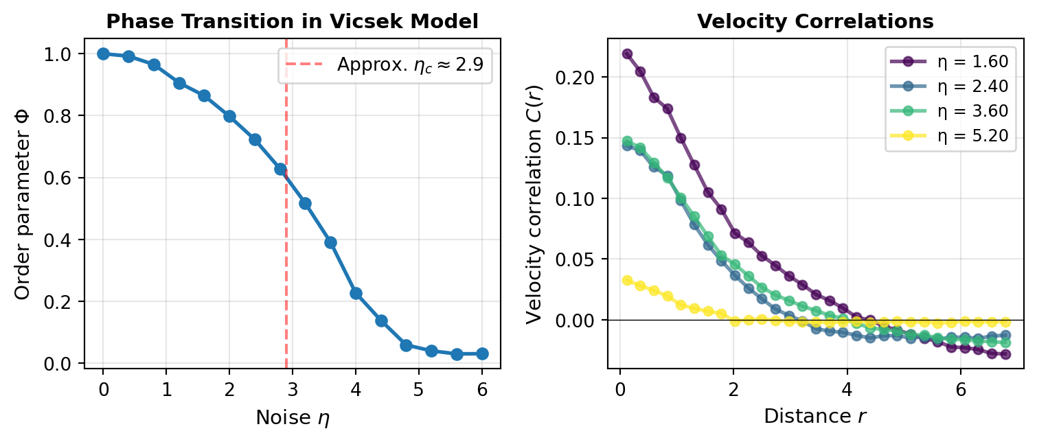
Figure 1— Velocity correlation functions in the Vicsek model. Left: Order parameter Φ versus noise η, showing the phase transition. Right: connected velocity-fluctuation correlation C(r) for several noise levels. The correlation length (the distance at which C(r) crosses zero) is large in the ordered phase (η < ηc ≈ 2.9) and collapses to a few interaction radii in the disordered phase.
This simulation demonstrates two key features:
Phase Transition: As noise increases, the system transitions from an ordered state (\(\Phi \approx 1\)) to a disordered state (\(\Phi \approx 0\)). For this density (\(\rho = N/L^2 = 5\)) the transition occurs near \(\eta_c \approx 2.9\). Here \(\eta\) is the width of the uniform angular noise interval (the original Vicsek convention), which is why \(\eta_c\) is larger than the dimensionless noise amplitude used in Lecture 7.
Correlations at Different Phases: The plotted \(C(r)\) is the connected correlation of velocity fluctuations (the mean flock velocity is subtracted), and it changes sign at a distance that measures the correlation length. In the ordered phase (\(\eta < \eta_c\)) the fluctuations stay correlated over large distances – the correlation length is comparable to the system size, the scale-free behavior seen in real flocks – while in the disordered phase (\(\eta > \eta_c\)) the correlation length collapses and \(C(r)\) decays to zero within a few interaction radii. The small negative dip at large \(r\) is a finite-size effect: because the global mean velocity is subtracted, the fluctuations of all particles must sum to zero, which forces the off-diagonal correlations to be slightly negative on average.
Maximum Entropy Models and Critical Behavior
Bialek et al. (2012) introduced a powerful framework for understanding collective motion: the maximum entropy principle. Given observed correlations in a real flock, what is the least-biased probability distribution consistent with those observations?
For a system where each particle has a direction (unit vector) \(\mathbf{s}_i = \mathbf{v}_i/|\mathbf{v}_i|\), the maximum entropy distribution with pairwise constraints takes the form of a Boltzmann distribution:
\(J_{ij}\) are coupling constants representing the strength of pairwise interactions (analogous to Ising model couplings)
\(\mathbf{h}_i\) are external field terms (like magnetic fields in magnetism)
\(Z\) is the partition function ensuring normalization
The model reproduces observed single-particle statistics (via \(\mathbf{h}_i\)) and pairwise correlations (via \(J_{ij}\))
Derivation: Maximum Entropy Principle
The maximum entropy principle states that among all probability distributions consistent with known constraints (like measured correlations), we should choose the one that maximizes entropy \(S = -\sum_x P(x) \ln P(x)\).
Maximizing yields the Boltzmann form with \(\mathbf{h}_i = \lambda_i\) and \(J_{ij}\) related to \(\Lambda_{ij}\).
A crucial finding: real flocks operate near critical points where the effective temperature (noise level) equals the critical temperature. This means flocks sit at the boundary between ordered and disordered phases, maximizing their susceptibility to perturbations. A small change (like a predator attack) can propagate instantaneously through the entire group because the system is poised at criticality.
This is not a coincidence—evolution has tuned biological systems to operate at critical points where information can propagate fastest and the system is most responsive.
Topological vs Metric Interactions
The distinction between metric interactions (each individual responds to every neighbor within a fixed radius \(R\)) and topological interactions (each responds to a fixed number \(k\) of nearest neighbors, irrespective of distance), together with the Voronoi construction used to define neighbors, was developed in Lecture 7. Here we focus on the experimental evidence and its biological significance.
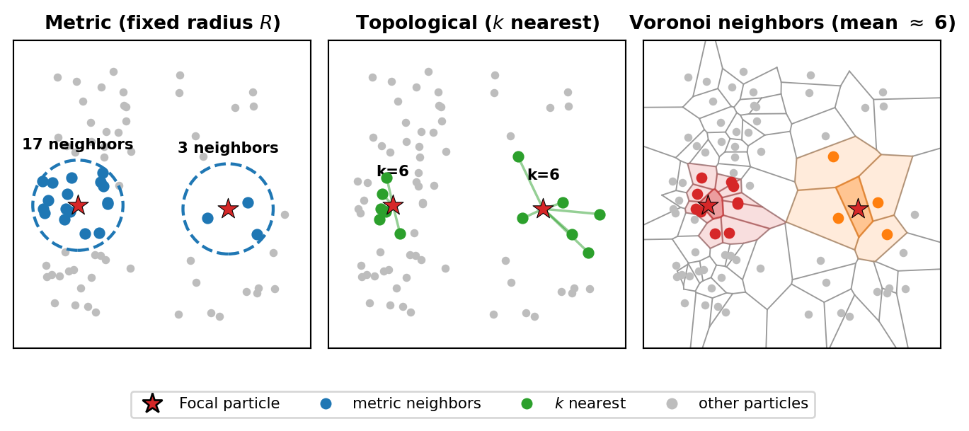
The STARFLAG experiments (Ballerini et al. 2008) demonstrated that starlings use topological interactions with approximately \(k \approx 6-7\) neighbors per bird, and Couzin et al. (2002) reached the same conclusion for fish. The metric, topological, and Voronoi neighborhoods are compared in Figure 2.
Code
import numpy as npimport matplotlib.pyplot as pltfrom matplotlib.lines import Line2Dfrom scipy.spatial import Voronoi# Point set with two regions: a dense cluster on the left, a sparse population# on the right. We compare how a focal particle in each region selects neighbors.np.random.seed(3)dense = np.random.rand(55, 2) * [3.5, 10] + [0.3, 0]sparse = np.random.rand(22, 2) * [4.5, 10] + [5.2, 0]pos = np.vstack([dense, sparse])def closest(target):returnint(np.argmin(np.linalg.norm(pos - np.array(target), axis=1)))focal_dense = closest([2.0, 5.0]) # focal particle in the dense regionfocal_sparse = closest([7.3, 5.0]) # focal particle in the sparse regionGREY ='#bdbdbd'; RED ='#d62728'; BLUE ='#1f77b4'; GREEN ='#2ca02c'; ORANGE ='#ff7f0e'R =1.7# metric interaction radiusk =6# number of topological neighborsfig, axes = plt.subplots(1, 3, figsize=(7.0, 3.0)) # 7.0 in = 17.8 cm wide# Panel 1: metric interactions -- same radius R for both focal particlesax = axes[0]ax.scatter(pos[:, 0], pos[:, 1], s=11, color=GREY, zorder=2)for fi in (focal_dense, focal_sparse): fp = pos[fi] d = np.linalg.norm(pos - fp, axis=1) nb = np.where((d < R) & (d >0))[0] ax.add_patch(plt.Circle(fp, R, fill=False, ec=BLUE, ls='--', lw=1.6, zorder=3)) ax.scatter(pos[nb, 0], pos[nb, 1], s=26, color=BLUE, zorder=4) ax.scatter(*fp, s=130, color=RED, marker='*', ec='k', lw=0.4, zorder=6) ax.annotate(f'{len(nb)} neighbors', (fp[0], fp[1] + R +0.4), ha='center', fontsize=8, fontweight='bold')ax.set_title('Metric (fixed radius $R$)', fontsize=10, fontweight='bold')# Panel 2: topological interactions -- k nearest neighbors for bothax = axes[1]ax.scatter(pos[:, 0], pos[:, 1], s=11, color=GREY, zorder=2)for fi in (focal_dense, focal_sparse): fp = pos[fi] d = np.linalg.norm(pos - fp, axis=1) knn = np.argsort(d)[1:k+1]for j in knn: ax.plot([fp[0], pos[j, 0]], [fp[1], pos[j, 1]], '-', color=GREEN, alpha=0.5, lw=1.3, zorder=3) ax.scatter(pos[knn, 0], pos[knn, 1], s=26, color=GREEN, zorder=4) ax.scatter(*fp, s=130, color=RED, marker='*', ec='k', lw=0.4, zorder=6) ax.annotate(f'k={k}', (fp[0], fp[1] +1.1), ha='center', fontsize=8, fontweight='bold')ax.set_title('Topological ($k$ nearest)', fontsize=10, fontweight='bold')# Panel 3: Voronoi tessellation -- topological neighbors are cells sharing an edgeax = axes[2]vor = Voronoi(pos)for rv in vor.ridge_vertices: rv = np.asarray(rv)if np.all(rv >=0): ax.plot(vor.vertices[rv, 0], vor.vertices[rv, 1], '-', color='#999999', lw=0.7, zorder=1)ax.scatter(pos[:, 0], pos[:, 1], s=11, color=GREY, zorder=2)def voronoi_neighbors(idx): nb =set()for a, b in vor.ridge_points:if a == idx: nb.add(b)elif b == idx: nb.add(a)returnlist(nb)def fill_cell(idx, color, alpha): region = vor.regions[vor.point_region[idx]]if region and-1notin region: poly = vor.vertices[region] ax.fill(poly[:, 0], poly[:, 1], color=color, alpha=alpha, zorder=1)for fi, col in ((focal_dense, RED), (focal_sparse, ORANGE)):for nb in voronoi_neighbors(fi): fill_cell(nb, col, 0.15) fill_cell(fi, col, 0.45) ax.scatter(pos[voronoi_neighbors(fi), 0], pos[voronoi_neighbors(fi), 1], s=24, color=col, zorder=4) ax.scatter(*pos[fi], s=130, color=RED, marker='*', ec='k', lw=0.4, zorder=6)# Average number of Voronoi neighbors over interior (bounded) cells is ~6 (Euler)bounded = [i for i inrange(len(pos))if vor.regions[vor.point_region[i]] and-1notin vor.regions[vor.point_region[i]]]mean_vn = np.mean([len(voronoi_neighbors(i)) for i in bounded])ax.set_title(f'Voronoi neighbors (mean $\\approx$ {mean_vn:.0f})', fontsize=10, fontweight='bold')for ax in axes: ax.set_xlim(-0.7, 10.5); ax.set_ylim(-0.7, 10.9); ax.set_aspect('equal') ax.set_xticks([]); ax.set_yticks([]) # positions are schematic; no axis numbers or labelslegend_items = [ Line2D([0], [0], marker='*', color='w', markerfacecolor=RED, markeredgecolor='k', markersize=11, label='Focal particle'), Line2D([0], [0], marker='o', color='w', markerfacecolor=BLUE, markersize=7, label='metric neighbors'), Line2D([0], [0], marker='o', color='w', markerfacecolor=GREEN, markersize=7, label='$k$ nearest'), Line2D([0], [0], marker='o', color='w', markerfacecolor=GREY, markersize=7, label='other particles'),]fig.legend(handles=legend_items, loc='lower center', ncol=4, fontsize=8, bbox_to_anchor=(0.5, -0.01), frameon=True)plt.tight_layout(pad=0.4)plt.subplots_adjust(bottom=0.13, wspace=0.06)plt.show()
Figure 2— Metric versus topological neighborhoods for a focal particle (red star) placed once in a dense region and once in a sparse region. Left: a fixed metric radius R captures a strongly density-dependent number of neighbors (many in the dense region, few in the sparse one). Middle: the k = 6 nearest neighbors are selected regardless of local density, so the interaction count is fixed and only the reach changes. Right: the Voronoi tessellation defines topological neighbors as cells sharing an edge; the average number of such neighbors is approximately 6, which is why k ≈ 6-7 is a natural choice.
This comparison illustrates why topological interactions are crucial for biological collectives:
Stability across density changes: a fixed metric radius captures a strongly density-dependent number of neighbors (many in the dense region, only a few in the sparse one, as the left panel shows), whereas the topological rule always uses the same \(k\).
Robustness: organisms need predictable interaction rules; the topological neighborhood provides this stability as the flock expands and contracts.
Why \(k \approx 6\): the average number of Voronoi neighbors of a point in the plane is exactly 6 (a consequence of Euler’s formula), so the measured \(k \approx 6-7\) for starlings is a natural value, and Voronoi neighbors are a good proxy for the interaction network.
Evolutionary origin: in visually-oriented animals, the \(k\) nearest neighbors correspond to the number of individuals that occupy the visual field at typical inter-individual spacing.
Information Propagation Speed and Sound Modes
In the ordered phase, directional changes propagate as waves through the group, with a linear (sound-like) dispersion relation \(\omega(k) = c_s k + O(k^2)\) rather than the diffusive spreading of the standard Vicsek model. The dispersion-relation derivation and the role of behavioral inertia were treated in detail in Lecture 7, and the full Toner-Tu hydrodynamic equations in Lecture 8; here we record the measured numbers for real flocks.
High-speed tracking of starling flocks (Attanasi et al. 2014, Nature Physics) measured:
Propagation speed of turning information: \(c_s \approx 20-40\) m/s
Individual bird flight speed: \(v_0 \approx 10-15\) m/s
Reaction time to a nearest neighbor: \(\tau \approx 50-100\) ms
The collective propagation speed is therefore substantially faster than nearest-neighbor relay alone would allow (\(c_s > v_0\)), signalling non-local information transfer: near criticality the correlation length extends far beyond nearest neighbors, so each bird effectively responds to perturbations from distant parts of the flock.
Fish Schools: Experimental Systems
Fish schools offer another striking example of collective motion, with some species forming schools comprising millions of individuals that move as a coordinated unit. These schools can rapidly change direction, split and reform, and create complex three-dimensional structures in response to environmental cues or predators.
In laboratory settings, researchers have created controlled environments to study schooling behavior quantitatively. Large tanks with overhead cameras track individual and group movements, while controlled stimuli such as simulated predators or food sources can be introduced to test response patterns.
For stunning visualizations of fish schooling behavior, see the videos in Tunstrøm et al. (2013, PLOS Computational Biology), which provide dynamic footage of golden shiners exhibiting various collective states (milling, swarming, and schooling). These videos are available in their supplementary materials and highlight the coordinated nature of fish movements even during rapid directional changes and transitions between states.
Studies on various fish species have revealed the fundamental mechanisms underlying schooling behavior. Extensive research on golden shiners (Notemigonus crysoleucas) by Katz et al. (2011) used automated tracking systems to analyze the movement patterns of individuals within schools. They identified three primary interaction rules governing collective motion: short-range repulsion to avoid collisions, intermediate-range alignment with neighbors’ directions, and longer-range attraction to maintain group cohesion. For excellent video demonstrations of these principles, see the Collective Dynamics Group at Princeton University (https://cdg.princeton.edu/research/) and the Couzin Lab at Max Planck Institute (https://collectivebehaviour.com/research/), which offer numerous videos of experimental setups similar to those used in Katz’s research.
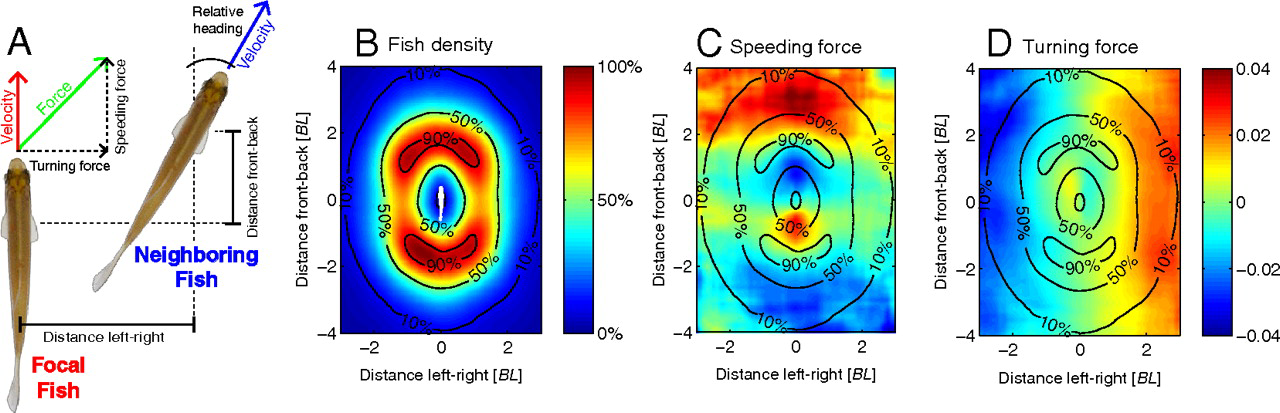
Figure 3— Two-fish configurations. (A) Diagram showing how a focal fish’s coordinate system is used to measure a neighbor’s relative position and heading. The focal fish’s acceleration is decomposed into speeding and turning components. (B) Probability distribution of finding the neighboring fish at different positions relative to the focal fish. Contours show 10%, 50%, and 90% probability levels. (C and D) Maps showing how a neighbor’s position affects the focal fish’s speeding and turning responses, respectively. In speeding forces, positive values indicate acceleration; in turning forces, positive values indicate right turns. Distances in body lengths [BL] and time in seconds [s]. Analysis excluded fish near boundaries or moving slowly. (see Katz et al. (2011))
Fish schools also respond collectively to environmental gradients. Berdahl et al. (2013, Science) demonstrated that golden shiners navigate light gradients more effectively as a group than as individuals, showing a form of emergent collective sensing. Their Figure 3 shows how schooling enhances gradient-tracking ability across different group sizes, with a clear diagram of performance improvement as group size increases.
The sensory mechanisms enabling schooling include both the lateral line system (detecting water pressure changes) and vision. Partridge and Pitcher (1980, Journal of Comparative Physiology) conducted pioneering experiments selectively disabling these sensory systems, showing that both contribute to different aspects of schooling behavior. Their paper illustrates how sensory impairment affects different components of schooling behavior.
Leadership in fish schools emerges dynamically based on information possession rather than from a fixed hierarchy. Strandburg-Peshkin et al. (2013, PNAS) showed that individuals with information about food location temporarily lead groups, with leadership shifting as information distributes. Their Figure 2 provides network diagrams showing how leadership networks reconfigure during these transitions.
Golden shiners have been extensively studied by Strandburg-Peshkin et al. (2013), who used high-resolution tracking to examine how visual field restrictions influence interaction networks within schools. They found that fish primarily respond to neighbors within their visual field, creating asymmetric interaction networks that nonetheless maintain group cohesion. Their Figure 3 provides a detailed visualization of these visual interaction networks, showing how spatial position relative to a fish’s heading affects its influence.
During predator evasion, information cascades through the group, creating what researchers call “escape waves.” Rosenthal et al. (2015, PNAS) documented this phenomenon, showing how startle responses propagate through schools with increasing speed as they travel. Their analysis provides space-time diagrams illustrating these cascades, with clear visualization of how information propagation accelerates through the group.
Zebrafish larvae demonstrate fascinating transitions between different collective states. Tunstrøm et al. (2013, PLOS Computational Biology) observed three distinct patterns of organization: schooling (polarized, directional movement), milling (rotating around an empty core), and disordered swarming. Their study shows these distinct states with velocity field overlays, while their observations provide a phase diagram showing transitions between states as a function of group size and tank size.
The Vicsek model has proven remarkably effective at capturing certain aspects of fish schooling behavior. The transitions between ordered and disordered motion observed in real fish schools closely resemble the phase transitions in the Vicsek model as noise parameters change. Gautrais et al. (2012, PLOS Computational Biology) demonstrated this correspondence, with their research showing a comparative phase diagram between model predictions and actual fish behavior data.
When boundary conditions are incorporated into Vicsek-type models, they can reproduce the milling behavior frequently observed in confined fish schools. Tunstrøm et al. (2013) successfully reproduced the schooling-milling-swarming transitions seen in real fish using a modified Vicsek model with boundary interactions. Their work provides side-by-side comparisons of experimental observations and simulation results, showing striking similarities in pattern formation.
Real fish exploit hydrodynamic effects in ways that go beyond simple Vicsek-like models. Fish swimming in diamond-shaped formations reduce drag by capturing vortices shed by fish ahead of them. Marras et al. (2015, Nature Communications) quantified these energy-saving effects, with their results showing flow visualization around fish in different positions within a school and the corresponding energy expenditure measurements.
Toner-Tu theory extensions that incorporate fluid dynamics interactions better match the experimental data on fish schools. Hemelrijk et al. (2015, Interface Focus) showed how hydrodynamic effects influence school structure, with their research illustrating how vortex capture leads to the specific spacing patterns observed in real schools.
Some clustering behavior in fish shows remarkable similarities to MIPS. Filella et al. (2018, Physical Review Letters) demonstrated density-dependent motility in certain fish species that leads to spontaneous clustering even without explicit attraction forces. Their study shows the density profiles in these clusters, closely matching predictions from MIPS theory.
Insect Swarms: Locusts
Locust swarms represent one of the most dramatic examples of collective motion with significant ecological and economic impact. During outbreaks, desert locusts (Schistocerca gregaria) can form swarms covering hundreds of square kilometers and containing billions of individuals, all moving in coordinated fashion across vast distances.
These massive swarms exhibit striking directional alignment, with all individuals traveling in approximately the same direction while maintaining a dense, cohesive group structure. The transition from solitary to swarming behavior in locusts represents a remarkable example of a density-dependent phase transition in biological systems.
For impressive visualization of locust collective motion, see the work of Buhl et al. (2006, Science), which presents time-lapse photography of locusts marching in aligned groups, alongside plots of their directional order parameters changing with density.
Laboratory studies by Buhl et al. (2006) used ring-shaped arenas to analyze locust movement patterns quantitatively. By confining locusts to an annular track, researchers could precisely control density while measuring directional order over extended periods. They discovered that locusts exhibit spontaneous direction switching, with the entire group occasionally reversing direction in a highly coordinated manner. The frequency of these switches decreases as density increases, eventually leading to stable unidirectional movement at high densities.
A key finding from these experiments was that the order parameter (a measure of directional alignment) depends strongly on density, with a critical transition point where the system shifts from disordered to ordered movement. Buhl’s research provides a clear diagram showing this relationship between density and order parameter, with a sharp transition region that closely resembles predictions from statistical physics models.
Field observations of locust swarms reveal massive directional migration covering hundreds of kilometers, with remarkable persistence in direction despite encountering diverse terrain and obstacles. Sword et al. (2010, Behavioral Ecology) documented these migration patterns using remote sensing and ground observations. Their study shows satellite tracking data of swarm movements over multiple days, demonstrating the extraordinary coherence of direction at landscape scales.
Perhaps most fascinating is the density-dependent phase transition from solitary to gregarious behavior in locusts. This behavioral phase change involves morphological, physiological, and behavioral modifications triggered by increased population density. Rogers et al. (2014, Advances in Insect Physiology) documented these changes, with their work illustrating how serotonin levels correlate with behavioral transitions across different density conditions.
The Vicsek model finds perhaps its most direct biological application in locust collective motion. The density-dependent order parameter observed in locust experiments matches the predictions of the Vicsek model with remarkable precision. Buhl et al. (2006) directly compared their experimental data with simulations, showing in their results how both systems exhibit similar phase transitions with increasing density.
Bistability and direction switching observed in both the model and experiments further strengthen this connection. Yates et al. (2009, PNAS) developed a modified Vicsek model that accurately reproduces the spontaneous direction switching seen in locust groups, with decreasing switch frequency as density increases. Their research provides a bifurcation diagram showing the transition from bistable to monostable dynamics in both real locusts and the model system.
Interestingly, cannibalism appears to be a driving force behind directional alignment in locusts. Bazazi et al. (2008, Current Biology) demonstrated that locusts move forward to avoid being eaten from behind by conspecifics, creating a directional bias that amplifies through the group. Their study shows experimental results where artificial reduction of cannibalistic behavior (through blocking mandibles) significantly reduces group alignment.
Models incorporating pursuit-escape dynamics better match experimental data than pure alignment models. Romanczuk et al. (2009, Physical Review Letters) developed an “escape-pursuit” model specifically for locusts that reproduces observed collective dynamics. Their work provides phase diagrams comparing standard Vicsek dynamics with pursuit-driven alignment, showing how the latter better matches the abrupt transitions observed in real locust groups.
Insect Swarms: Ants
Ant colonies demonstrate collective motion patterns distinct from those seen in other systems, primarily through their formation of trail networks. Rather than aligning directly with each other like birds or fish, ants coordinate through indirect interactions mediated by pheromone deposition on the environment.
This pheromone-based system creates self-reinforcing pathways where initial random exploration leads to optimal transport networks through positive feedback. Frequently used trails receive more pheromone, attracting more ants, while less-used paths fade as pheromones evaporate, eventually converging on efficient solutions to complex problems.
For visual representation of ant trail formation, see the research by Perna et al. (2012, Journal of the Royal Society Interface), which shows time-lapse photography of trail development alongside pheromone concentration maps reconstructed from ant traffic patterns.
The theoretical connection to collective motion differs from direct alignment models like Vicsek. Ant systems are better modeled as active Brownian particles with trail interactions, where individuals modify their environment, which in turn influences subsequent behavior. This creates a memory effect absent in Vicsek-type models.
Deneubourg et al. (1989, Journal of Theoretical Biology) provided the classic “double bridge” experiment demonstrating how this simple mechanism leads to collective decision-making. Their work shows the experimental setup and results, where the colony collectively selects the shorter of two paths through pheromone amplification.
These distinct interaction mechanisms highlight how different biological systems have evolved various strategies for collective coordination, all achieving robust group behavior through different means. Reid et al. (2015, PNAS) compared different collective decision-making mechanisms across species, with their study providing a comparative diagram of direct versus indirect coordination systems.
Cellular Systems: Bacterial Colonies
At the microscopic scale, bacterial colonies provide fascinating examples of collective motion with important connections to theoretical models. Dense bacterial suspensions can self-organize into complex dynamic patterns including jets, vortices, and turbulent-like flows despite the simplicity of the individual cells.
These patterns emerge from the interplay between cell motility, cell shape, and environmental factors, creating rich collective dynamics that have become an important model system in active matter physics. The small size and rapid reproduction of bacteria make them ideal for controlled experiments on collective motion.
For striking visualizations of bacterial collective motion, see the research by Zhang et al. (2010, PNAS), which shows time-lapse microscopy of B. subtilis colonies with velocity field overlays, revealing the flow patterns that emerge spontaneously in these active suspensions.
Collective motion observed under the density condition of N=718. The field of view is 90 × 90 μm2. Source: PNAS
Bacillus subtilis has been extensively studied by Zhang et al. (2010) and Peruani et al. (2012, Physical Review Letters), who documented how high-density bacterial suspensions form dynamic patterns of jets and vortices. Using microscopy and particle tracking, they observed that these rod-shaped bacteria align their bodies due to physical constraints (nematic alignment) rather than actively seeking to match their neighbors’ directions.
At high densities, B. subtilis suspensions develop turbulent-like flows with characteristic swirling patterns and jets spanning multiple cell lengths. Chen et al. (2017, PNAS) characterized these flows quantitatively, showing in their analysis how the statistical properties of bacterial turbulence differ from conventional fluid turbulence, with distinct energy spectra and correlation functions.
Escherichia coli exhibits different collective dynamics based on its run-and-tumble motion pattern. Berg’s classic work characterized the individual movement strategy, while Di Leonardo et al. (2010, PNAS) examined how these movements lead to collective behavior. Their research demonstrates how run-and-tumble statistics change in dense populations, leading to effective long-range interactions through the fluid.
Chemotaxis—the directed movement toward or away from chemical gradients—strongly influences bacterial collective behavior. Park et al. (2003, Science) showed how E. coli populations form complex patterns when responding to self-generated nutrient gradients. Their results provide time-series images of pattern formation dependent on nutrient concentration, with accompanying diagrams explaining the feedback mechanisms responsible.
Active nematic models better describe rod-shaped bacteria than Vicsek-type models that assume polar alignment. This is because elongated bacteria primarily align their bodies (axes) without necessarily matching their direction of movement. Doostmohammadi et al. (2018, Nature Communications) demonstrated this connection, with their work comparing experimental observations of bacterial suspensions with active nematic simulations, showing remarkable similarities in defect formation and dynamics.
These bacterial systems exhibit topological defects—singularities in the orientation field—that are predicted by active nematic theory. Kawaguchi et al. (2017, Nature) directly observed these defects in bacterial colonies and showed how they influence colony dynamics. Their study shows microscopy images of +1/2 and -1/2 defects in bacterial colonies alongside theoretical predictions of defect structure.
MIPS (Motility-Induced Phase Separation) manifests clearly in active systems. Buttinoni et al. (2013, Physical Review Letters) demonstrated how density-dependent motility leads to spontaneous clustering even without explicit attraction in synthetic self-propelled Janus particles. Their research shows experimental measurements of density profiles in these active colloid clusters alongside predictions from MIPS theory, highlighting the quantitative agreement between theory and observation. Similar phenomena have been observed in bacterial systems by Theurkauff et al. (2012, Physical Review Letters).
Models incorporating quorum sensing—bacteria’s ability to detect local population density through chemical signals—successfully capture complex clustering behaviors. Liu et al. (2019, Physical Review Letters) developed models combining MIPS with quorum sensing, with their results showing phase diagrams of different collective states as functions of sensing parameters and motility.
Cross-Species Comparison
System
Interaction Type
Order Parameter
Match to Theory
Birds
Topological alignment
Polarization
Vicsek + topological
Fish
Visual alignment + hydrodynamics
Polarization, milling
Vicsek + boundaries
Locusts
Cannibalistic pursuit
Polarization
Vicsek + pursuit
Bacteria
Nematic alignment
Nematic order
Active nematics, MIPS
For visual comparisons across different collective systems, see the comprehensive work of Vicsek & Zafeiris (2012, Physics Reports), which provides side-by-side images of different biological systems alongside their velocity field reconstructions, highlighting similarities and differences in pattern formation.
Universal Features
Despite the diversity of biological collectives, several features recur across organisms and scales:
Order-disorder transitions controlled by density, noise, and interaction strength (Vicsek & Zafeiris, 2012).
Density thresholds for the onset of ordered motion, in locusts (Buhl et al., 2006), fish (Tunstrøm et al., 2013), and bacteria (Zhang et al., 2010).
Scale-free correlations in the ordered state (Cavagna et al., 2010; Herbert-Read et al., 2011), signalling proximity to a critical point.
Self-organized criticality, systems tuning themselves toward the critical point that maximizes responsiveness (Bialek et al., 2012).
Rapid, sound-like information transfer enabling collective response to threats (Attanasi et al., 2014; Rosenthal et al., 2015).
Theoretical Insights from Experiments
Experiments have mostly confirmed the Vicsek, Toner-Tu, and MIPS predictions and identified the extensions that real systems require. Bird-flock data revealed topological rather than metric interactions (Ballerini et al., 2008); confined fish schools showed boundary-induced milling states (Tunstrøm et al., 2013); and environmental gradients call for taxis terms beyond pure alignment (Berdahl et al., 2013). Direct measurements of turning waves in starling flocks (Attanasi et al., 2014; Cavagna et al., 2015) confirmed the linear sound modes and the 2D long-range order predicted by Toner-Tu theory, while density profiles in self-propelled colloids and bacteria (Buttinoni et al., 2013; Sokolov et al., 2018; Peruani et al., 2012) confirmed motility-induced phase separation and the role of persistence.
Methodology: Tracking Collective Motion
Quantitative study rests on tracking methods: 2D particle and optical-flow tracking for dense groups (Delcourt et al., 2013; Dell et al., 2014), multi-camera 3D reconstruction for flocks and schools (the STARFLAG system; Attanasi et al., 2015; Strandburg-Peshkin et al., 2013), and analysis of the resulting trajectories through correlation functions, order parameters for the different collective states (polarization, rotation, disorder; Tunstrøm et al., 2013), and interaction-network inference (Cavagna et al., 2010; Strandburg-Peshkin et al., 2013).
Current Challenges
Several challenges are shared across systems: individual heterogeneity (real animals are not identical particles; Jolles et al., 2017); multiple simultaneous interaction channels such as vision combined with the lateral line in fish (Strandburg-Peshkin et al., 2013); coupling to the environment through gradients, obstacles, and boundaries (Berdahl et al., 2013); the multi-scale link from individual sensing to group behavior (Sumpter et al., 2012); and the transient dynamics of state-to-state transitions, which often carry more information than the steady states themselves (Romensky et al., 2014).
Future Directions
Active directions include data-driven inference of interaction rules by machine learning, without preimposed structure (Heras et al., 2019); evolutionary accounts of why particular coordination strategies arise in different lineages (Ioannou, 2017); hybrid bio-robotic experiments that test interaction hypotheses directly by inserting programmed robots into animal groups (Bonnet et al., 2018); and the transfer of these principles to swarm robotics and human-crowd dynamics (Hamann, 2018).
Biological collective behavior shows remarkable diversity but also universal features across systems as different as bird flocks, fish schools, insect swarms, and bacterial colonies.
Simple theoretical models like Vicsek, Toner-Tu, and MIPS capture key aspects of these systems but require specific extensions to match the complexities of real biological collectives. These extensions – incorporating topological interactions, environmental responses, and system-specific behavioral rules – have significantly advanced our understanding.
Experimental observations continue to provide crucial insights for theory development, with increasingly sophisticated tracking and analysis methods revealing previously hidden aspects of collective dynamics.
The field exemplifies successful interdisciplinary collaboration, bringing together biology, physics, computer science, and mathematics to understand one of nature’s most spectacular phenomena.
Cavagna, A., et al. (2010). Scale-free correlations in starling flocks. PNAS, 107(26), 11865-11870.
Ballerini, M., et al. (2008). Interaction ruling animal collective behavior depends on topological rather than metric distance. PNAS, 105(4), 1232-1237.
Attanasi, A., et al. (2014). Information transfer and behavioural inertia in starling flocks. Nature Physics, 10(9), 691-696.
Bialek, W., et al. (2012). Statistical mechanics for natural flocks of birds. PNAS, 109(13), 4786-4791.
Herbert-Read, J.E., et al. (2011). Inferring the rules of interaction of shoaling fish. PNAS, 108(46), 18726-18731.
Katz, Y., et al. (2011). Inferring the structure and dynamics of interactions in schooling fish. PNAS, 108(46), 18720-18725.
Tunstrøm, K., et al. (2013). Collective states, multistability and transitional behavior in schooling fish. PLOS Computational Biology, 9(2), e1002915.
Strandburg-Peshkin, A., et al. (2013). Visual sensory networks and effective information transfer in animal groups. Current Biology, 23(17), R709-R711.
Berdahl, A., et al. (2013). Emergent sensing of complex environments by mobile animal groups. Science, 339(6119), 574-576.
Gautrais, J., et al. (2012). Deciphering interactions in moving animal groups. PLOS Computational Biology, 8(9), e1002678.
Buhl, J., et al. (2006). From disorder to order in marching locusts. Science, 312(5778), 1402-1406.
Bazazi, S., et al. (2008). Collective motion and cannibalism in locust migratory bands. Current Biology, 18(10), 735-739.
Yates, C.A., et al. (2009). Inherent noise can facilitate coherence in collective swarm motion. PNAS, 106(14), 5464-5469.
Perna, A., et al. (2012). Individual rules for trail pattern formation in Argentine ants (Linepithema humile). PLOS Computational Biology, 8(7), e1002592.
Zhang, H.P., et al. (2010). Collective motion and density fluctuations in bacterial colonies. PNAS, 107(31), 13626-13630.
Peruani, F., et al. (2012). Collective motion and nonequilibrium cluster formation in colonies of gliding bacteria. Physical Review Letters, 108(9), 098102.
Buttinoni, I., et al. (2013). Dynamical clustering and phase separation in suspensions of self-propelled colloidal particles. Physical Review Letters, 110(23), 238301.
Theurkauff, I., et al. (2012). Dynamic clustering in active colloidal suspensions with chemical signaling. Physical Review Letters, 108(26), 268303.
Sokolov, A., et al. (2018). Emergence of radial tree of bend stripes in active nematics. Physical Review X, 8(3), 031053.
Cates, M.E., & Tailleur, J. (2015). Motility-induced phase separation. Annual Review of Condensed Matter Physics, 6(1), 219-244.
Doostmohammadi, A., et al. (2018). Active nematics. Nature Communications, 9(1), 3246.
Sumpter, D.J.T. (2006). The principles of collective animal behaviour. Philosophical Transactions of the Royal Society B, 361(1465), 5-22.
Rosenthal, S.B., Twomey, C.R., Hartnett, A.T., Wu, H.S., & Couzin, I.D. (2015). Revealing the hidden networks of interaction in mobile animal groups. Proceedings of the National Academy of Sciences, 112(15), 4690-4695.
Park, S., Wolanin, P.M., Yuzbashyan, E.A., Silberzan, P., Stock, J.B., & Austin, R.H. (2003). Motion to form a quorum. Science, 301(5630), 188.