This page was generated from notebooks/L13/2_deep_learning_keras.ipynb.
![]()
You can directly download the pdf-version of this page using the link below.
download
Neural Network with Keras#
We have made a lot of effort to program our neural network that is able to classify differenr handwritten number with the help of numpy. A lot of other people did that already and since this is the basis for many applications nowadays, a large number of API (application programming interfaces) exist. Python plays therby a leading role. We will use in the follwing the interface provided by the keras module. keras is actually sitting on top of the real machine learning API, which is in our
case tensorflow. keras makes the use of tensorflow a bit more friendly and from the example below, you wil recognize by how much shorter our code gets with the keras and tensorflow API.
[31]:
from tensorflow.keras.datasets import mnist
from tensorflow.keras.utils import to_categorical,plot_model

from keras import Sequential
from keras.layers import Dense

import numpy as np
import matplotlib.pyplot as plt

%matplotlib inline
%config InlineBackend.figure_format = 'retina'

plt.rcParams.update({'font.size': 18,
                     'axes.titlesize': 20,
                     'axes.labelsize': 20,
                     'axes.labelpad': 1,
                     'lines.linewidth': 2,
                     'lines.markersize': 10,
                     'xtick.labelsize' : 18,
                     'ytick.labelsize' : 18,
                     'xtick.top' : True,
                     'xtick.direction' : 'in',
                     'ytick.right' : True,
                     'ytick.direction' : 'in'
                    })
MNIST Data Set (Keras)#
This loads the same data as in our previous notebook, except that the function to do that is directly provided by keras.
[32]:
(x_train, y_train), (x_test, y_test) = mnist.load_data()

x_train = x_train.reshape((60000, 28*28))
x_train = x_train.astype('float32')/255

x_test = x_test.reshape((10000, 28*28))
x_test = x_test.astype('float32')/255

# one-hot encoding
y_train = to_categorical(y_train)
y_test = to_categorical(y_test)
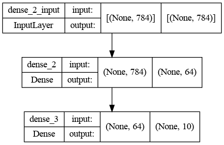
Build the model#
The next few lines create the whole neural network with an input layer, a hidden layer with 64 neurons and and output layer with 10 neurons.
[33]:
model = Sequential([
    Dense(64, activation='sigmoid', input_shape=(28 * 28, )),
    Dense(10, activation='softmax')
])
[34]:
plot_model(
    model,
    to_file='model.png',
    show_shapes=True,
    show_dtype=False,
    show_layer_names=True,
    rankdir='TB',
    expand_nested=False,
    dpi=96,
    layer_range=None,
    show_layer_activations=False
)
[34]:
Compile the model#
The compile method assembles everything to create a model for training. You can specify here the stochastic gradient descent method in the same way as the loss function.
[35]:
model.compile(optimizer='SGD',
              loss='categorical_crossentropy',
              metrics=['accuracy'])
Train the model#
Finally, the fit method allows us to train the model for a specified number of epochs.
[36]:
model.fit(x_train, y_train, epochs=20)
2024-07-02 06:42:01.092746: W tensorflow/core/framework/cpu_allocator_impl.cc:82] Allocation of 188160000 exceeds 10% of free system memory.
Epoch 1/20
1875/1875 [==============================] - 2s 805us/step - loss: 1.5565 - accuracy: 0.6634
Epoch 2/20
1875/1875 [==============================] - 2s 813us/step - loss: 0.7775 - accuracy: 0.8414
Epoch 3/20
1875/1875 [==============================] - 1s 573us/step - loss: 0.5627 - accuracy: 0.8687
Epoch 4/20
1875/1875 [==============================] - 1s 573us/step - loss: 0.4732 - accuracy: 0.8817
Epoch 5/20
1875/1875 [==============================] - 1s 634us/step - loss: 0.4237 - accuracy: 0.8890
Epoch 6/20
1875/1875 [==============================] - 1s 621us/step - loss: 0.3920 - accuracy: 0.8945
Epoch 7/20
1875/1875 [==============================] - 1s 665us/step - loss: 0.3694 - accuracy: 0.8991
Epoch 8/20
1875/1875 [==============================] - 1s 669us/step - loss: 0.3522 - accuracy: 0.9028
Epoch 9/20
1875/1875 [==============================] - 1s 665us/step - loss: 0.3387 - accuracy: 0.9055
Epoch 10/20
1875/1875 [==============================] - 1s 663us/step - loss: 0.3275 - accuracy: 0.9086
Epoch 11/20
1875/1875 [==============================] - 1s 655us/step - loss: 0.3180 - accuracy: 0.9105
Epoch 12/20
1875/1875 [==============================] - 1s 568us/step - loss: 0.3096 - accuracy: 0.9129
Epoch 13/20
1875/1875 [==============================] - 1s 631us/step - loss: 0.3023 - accuracy: 0.9150
Epoch 14/20
1875/1875 [==============================] - 1s 666us/step - loss: 0.2955 - accuracy: 0.9161
Epoch 15/20
1875/1875 [==============================] - 1s 667us/step - loss: 0.2894 - accuracy: 0.9179
Epoch 16/20
1875/1875 [==============================] - 1s 667us/step - loss: 0.2838 - accuracy: 0.9196
Epoch 17/20
1875/1875 [==============================] - 1s 730us/step - loss: 0.2785 - accuracy: 0.9209
Epoch 18/20
1875/1875 [==============================] - 1s 770us/step - loss: 0.2736 - accuracy: 0.9218
Epoch 19/20
1875/1875 [==============================] - 1s 719us/step - loss: 0.2687 - accuracy: 0.9235
Epoch 20/20
1875/1875 [==============================] - 1s 569us/step - loss: 0.2643 - accuracy: 0.9250
[36]:
<keras.callbacks.History at 0x7f08a499bc40>
Testing the model#
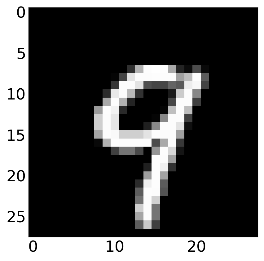
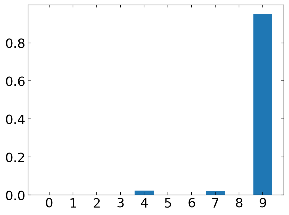
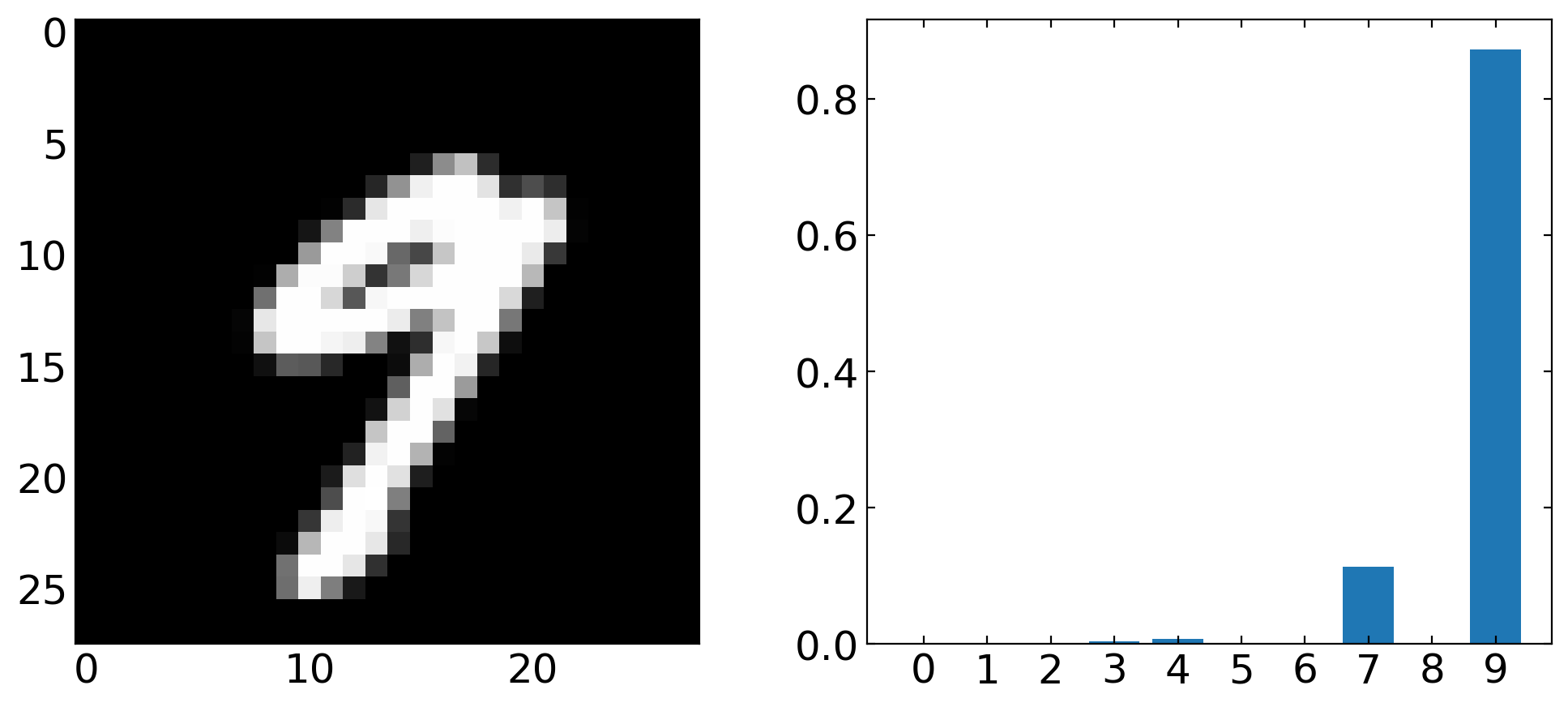
We may now use our trained model to predict the number in the image with the model.predict function. This delivers an array of 10 numbers, which represent the confidences that the number \(0,\ldots,9\) are contained. The index of the biggest number thus represents the number contained in the image.
[37]:
i = 12
plt.imshow(x_test[i,:].reshape(28,28), cmap='gray')
plt.show()
[38]:
model.predict(x_test[i,:].reshape(1,784))
[38]:
array([[7.1246905e-05, 1.8826446e-05, 2.5357914e-04, 6.1357114e-04,
        2.2916988e-02, 6.8956125e-04, 4.3461991e-05, 2.1728536e-02,
        1.9466790e-03, 9.5171756e-01]], dtype=float32)
[39]:
plt.bar( list(range(0,10)), model.predict(x_test[i,:].reshape(1,784))[0] )
plt.xticks( list(range(0,10)))
plt.show()
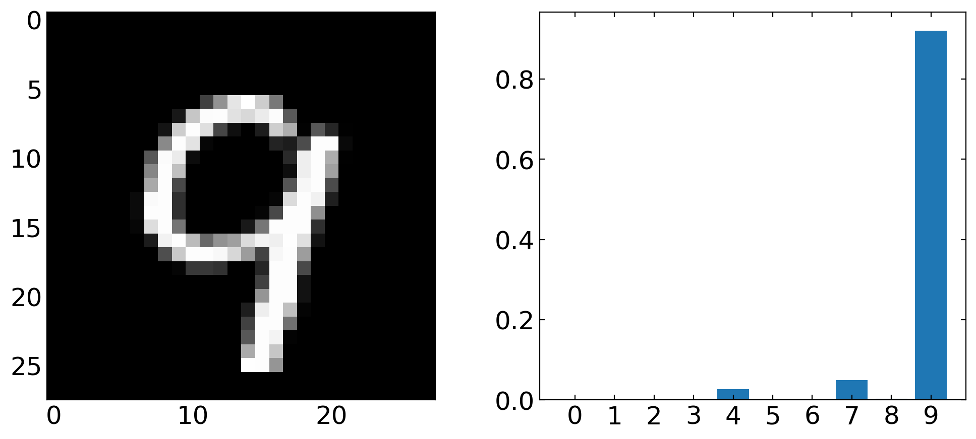
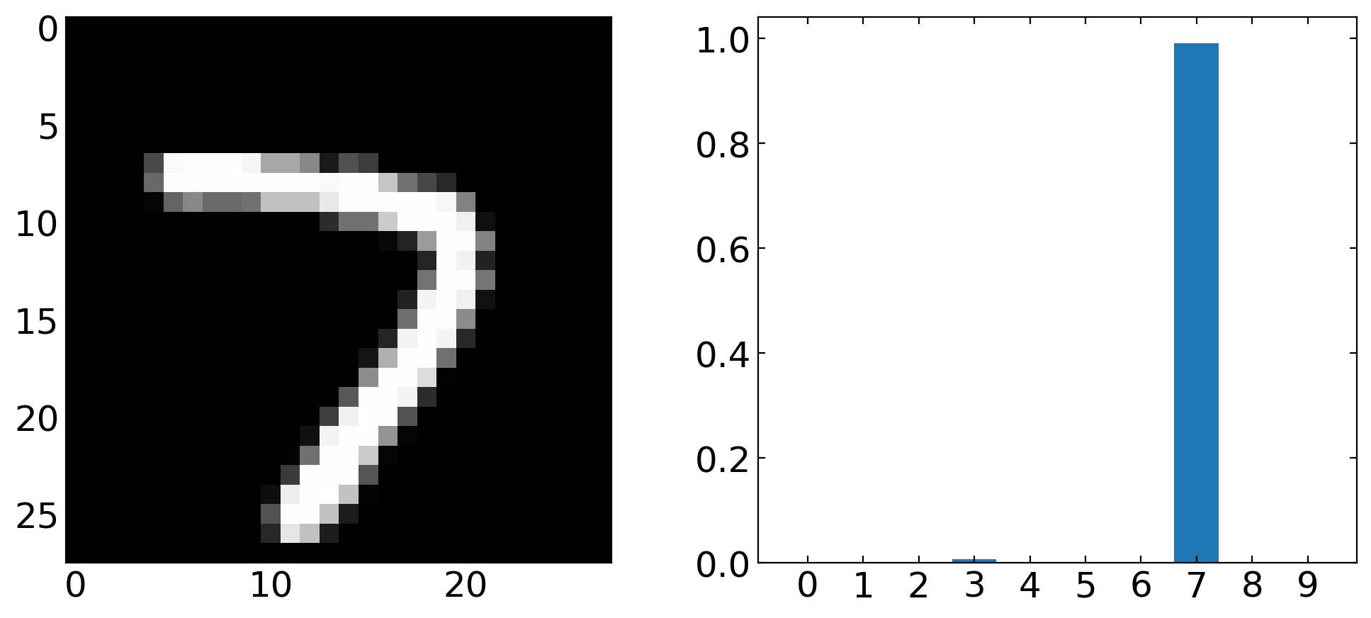
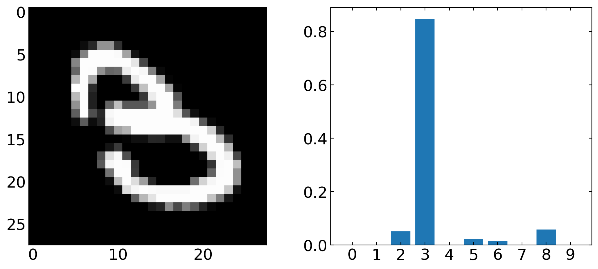
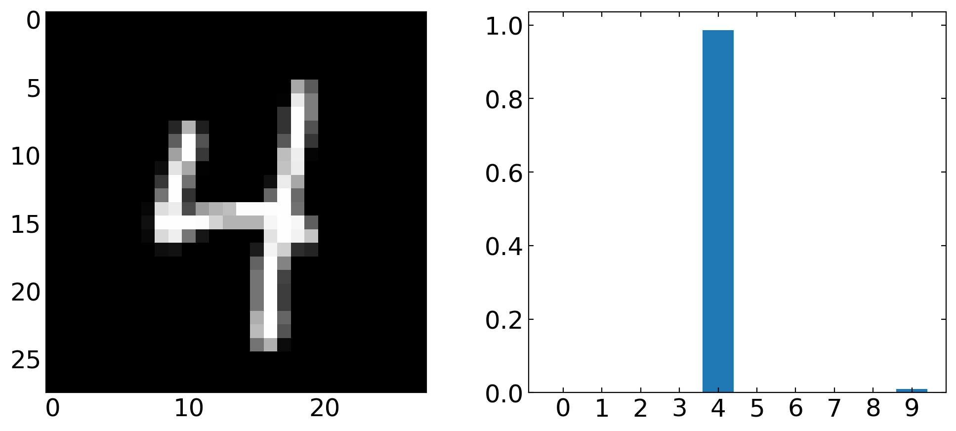
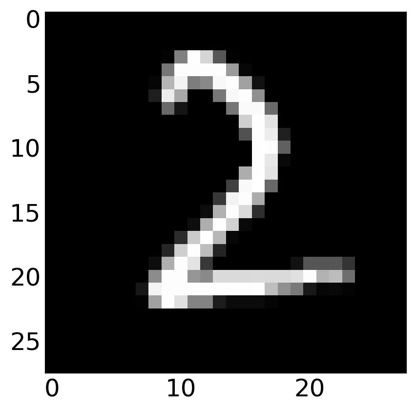
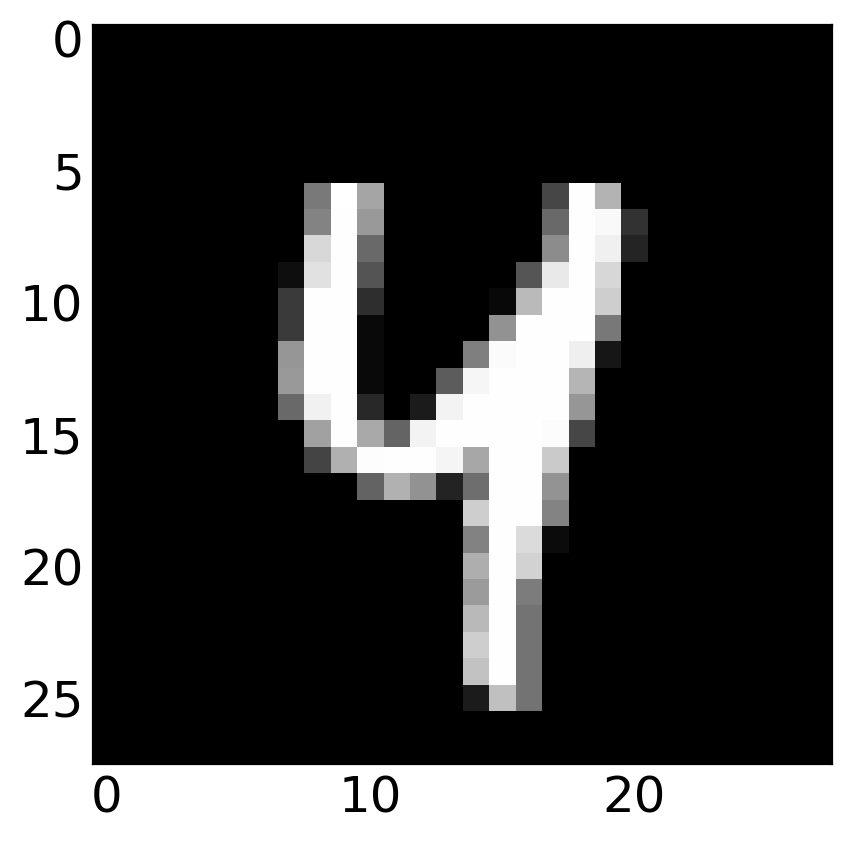
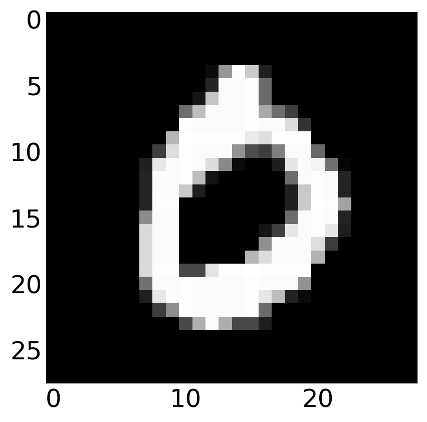
[10]:
for i in range(15,21):
    fig,axs = plt.subplots(1,2,figsize=(12,5))

    student = x_test[i,:].reshape(28,28)

    axs[0].imshow(student, cmap='gray')
    axs[1].bar( list(range(0,10)), model.predict(student.reshape(1,784))[0])
    axs[1].set_xticks(list(range(0,10)))

    plt.show()
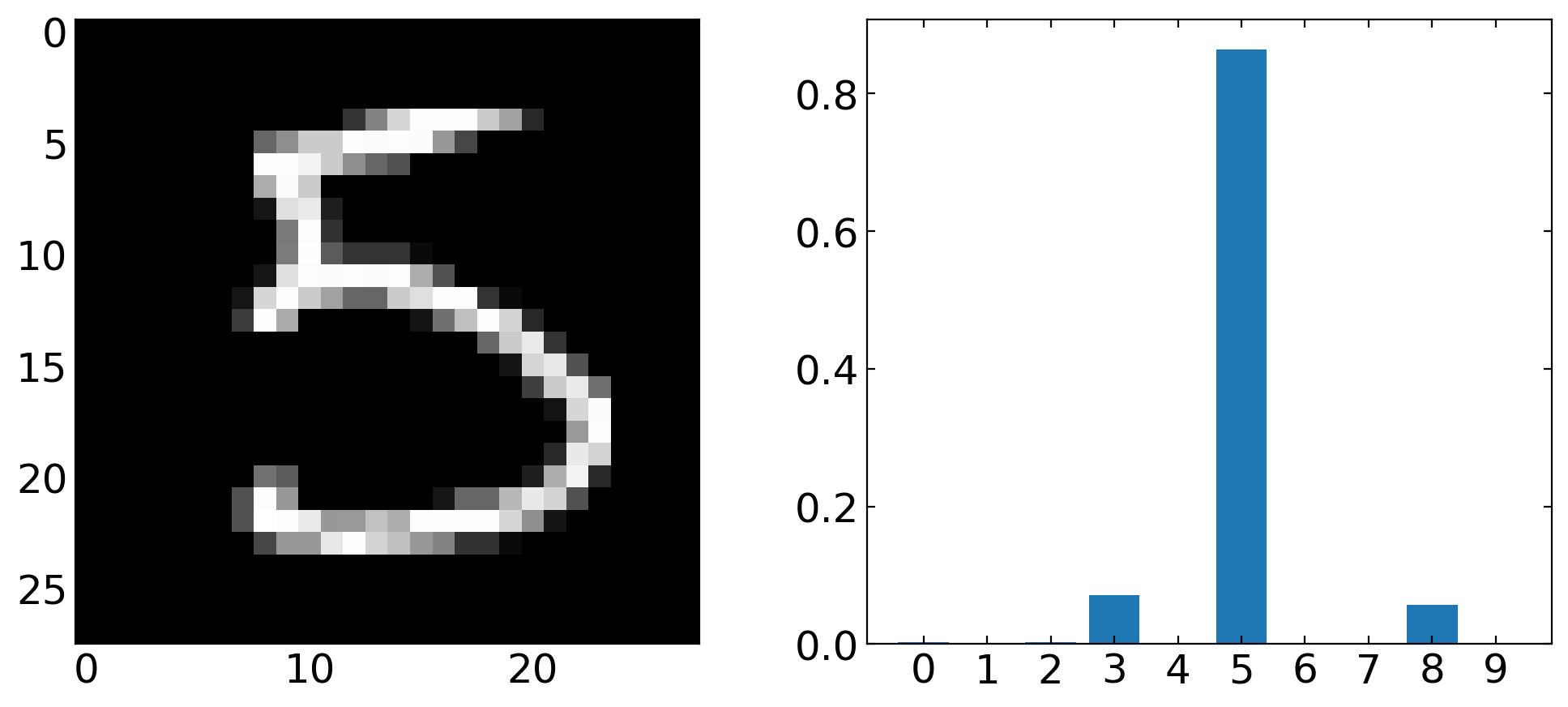
Testing with blended images
[21]:
i=42
[22]:
student=(x_test[i,:].reshape(28,28)+x_test[42,:].reshape(28,28)+x_test[3,:].reshape(28,28))/3
[23]:
plt.imshow(x_test[512,:].reshape(28,28),cmap="gray")
[23]:
<matplotlib.image.AxesImage at 0x7f08a49b2640>
[24]:
plt.imshow(x_test[42,:].reshape(28,28),cmap="gray")
[24]:
<matplotlib.image.AxesImage at 0x7f08a4b2a7f0>
[25]:
plt.imshow(x_test[3,:].reshape(28,28),cmap="gray")
[25]:
<matplotlib.image.AxesImage at 0x7f08a4b8fb50>
[26]:
plt.imshow(student,cmap="gray")
[26]:
<matplotlib.image.AxesImage at 0x7f08a435e490>

[27]:
plt.bar( list(range(0,10)), model.predict(student.reshape(1,784))[0] )
plt.xticks( list(range(0,10)))
plt.show()

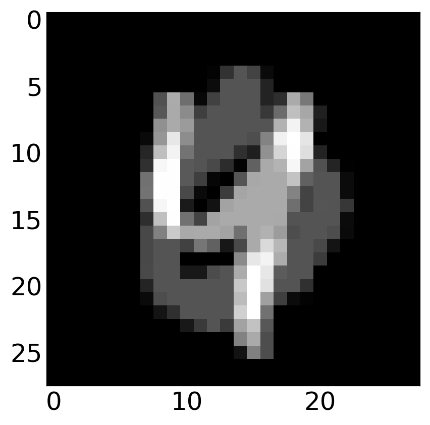
[28]:
i=42
student=(x_test[i,:].reshape(28,28)+x_test[42,:].reshape(28,28)+x_test[3,:].reshape(28,28))/3
plt.imshow(student.reshape(28,28), cmap='gray')
print("prediction: ",np.argmax(model.predict(student.reshape(1,784))))
prediction: 9
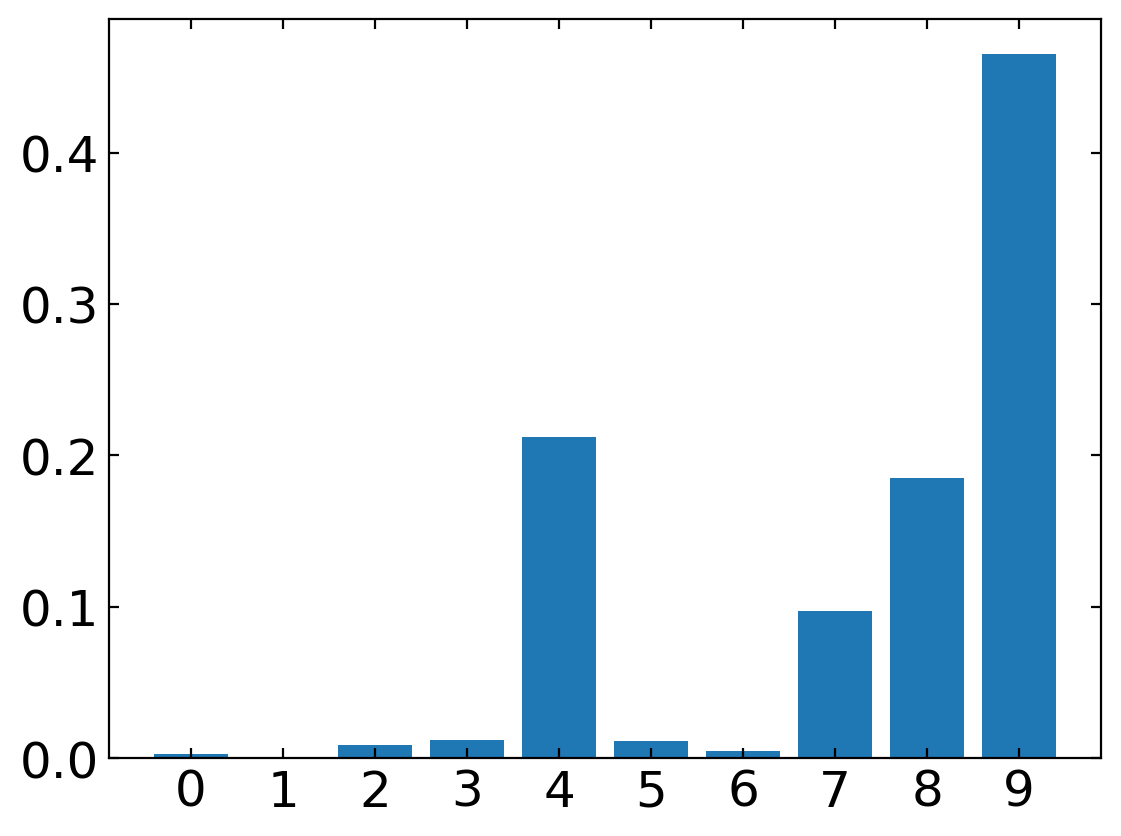
[29]:
model.predict(student.reshape(1,784))
[29]:
array([[0.00297183, 0.0006936 , 0.00873849, 0.01224055, 0.21193112,
        0.01138598, 0.00465778, 0.09701927, 0.18540345, 0.46495792]],
      dtype=float32)
[30]:
plt.bar( list(range(0,10)), model.predict(student.reshape(1,784))[0] )
plt.xticks( list(range(0,10)))
plt.show()
[ ]: