This page was generated from notebooks/L5/1_differentiation.ipynb.
![]()
You can directly download the pdf-version of this page using the link below.
download
Numerical Differentiation#
We did already have a look at the numerical differentiation in Lecture 3. We therefore don’t have to extend that to much here. Yet we want to formalize the numerical differentiation a bit.
[1]:
import numpy as np
import matplotlib.pyplot as plt

%matplotlib inline
%config InlineBackend.figure_format = 'retina'

plt.rcParams.update({'font.size': 10,
                     'lines.linewidth': 1,
                     'lines.markersize': 5,
                     'axes.labelsize': 10,
                     'xtick.labelsize' : 9,
                     'ytick.labelsize' : 9,
                     'legend.fontsize' : 8,
                     'contour.linewidth' : 1,
                     'xtick.top' : True,
                     'xtick.direction' : 'in',
                     'ytick.right' : True,
                     'ytick.direction' : 'in',
                     'figure.figsize': (4, 3),
                     'figure.dpi': 150 })
First order derivative#
Our previous way of finding the derivative was based on its definition
\begin{equation} f^{\prime}(x)=\lim_{\Delta x \rightarrow 0}\frac{f(x+x_{0})-f(x)}{\Delta x} \end{equation}
such that, if we don’t take the limit we can approximate the derivative by
\begin{equation} f^{\prime}_{i}\approx \frac{f_{i+1}-f_{i}}{\Delta x} \end{equation}
Here we look to the right of the current posiiton \(i\) and devide by the interval \(\Delta x\).
It is not difficult to see that the resulting local error \(\delta\) at each step is given by
Some better expression may be found by the Taylor expansion:
\begin{equation} f(x)=f(x_{0})+(x-x_0)f^{\prime}(x)+\frac{(x-x_0)^2}{2!}f^{\prime\prime}(x)+\frac{(x-x_0)^3}{3!}f^{(3)}(x)+\ldots \end{equation}
which gives in discrete notation
\begin{equation} f_{i+1}=f_{i}+\Delta x f_{i}^{\prime}+\frac{\Delta x^2 }{2!}f_{i}^{\prime\prime}+\frac{\Delta x^3 }{3!}f_{i}^{(3)}+\ldots \end{equation}
The same can be done to obtain the function value at \(i-1\)
\begin{equation} f_{i-1}=f_{i}-\Delta x f_{i}^{\prime}+\frac{\Delta x^2 }{2!}f_{i}^{\prime\prime}-\frac{\Delta x^3 }{3!}f_{i}^{(3)}+\ldots \end{equation}
which when neglecting the last term on the right side yields
\begin{equation} f^{\prime}_{i}\approx \frac{f_{i+1}-f_{i-1}}{2\Delta x} \end{equation}
This is similar to the formula we obtained from the definition of the derivative. Here, however, we use the function value to the left and the right of the position \(i\) and twice the interval, which actually improves accuracy.
[3]:
def D(f, x, h=1.e-4, *params):
    return (f(x+h, *params)-f(x-h, *params))/(2*h)
[9]:
def D1(f, x, h=1.e-4, *params):
    return (f(x+h, *params)-f(x, *params))/(h)
One may continue that type of derivation now to obtain higher order approximation of the first derivative with better accuracy. For that purpose you may calculate now \(f_{i\pm 2}\) and combining that with \(f_{i+1}-f_{i-1}\) will lead to
\begin{equation} f_{i}^{\prime}=\frac{1}{12 \Delta x}(f_{i-2}-8f_{i-1}+8f_{i+1}-f_{i+2}) \end{equation}
This can be used to give better values for the first derivative.
[4]:
def f(x):
    return(np.sin(x))
[5]:
x=np.linspace(0.01,np.pi*4,1000)
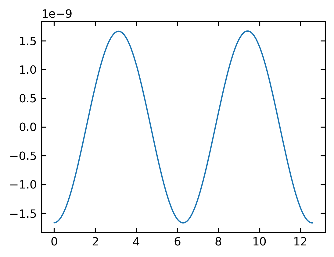
[11]:
#plt.plot(x,f(x))
plt.plot(x,D(f,x)-np.cos(x))
#plt.ylim(-2000,2000)
[11]:
[<matplotlib.lines.Line2D at 0x7fa9147624c0>]
Matrix version of the first derivative#
If we supply to the above function an array of positions \(x_{i}\) at which we would like to calculate the derivative, then we obtain and array of derivative values. We can write this procedure also in a different way, which will be helpful for solving differential equation later.
If we consider the above finite difference formulas for a set of positions \(x_{i}\), we can represent the first derivative at these positions by matrix operation as well:
\(f^{\prime}=\frac{1}{\Delta x} \begin{bmatrix} -1 & 1 & 0 & 0 & 0 & 0\\ 0 & -1 & 1 & 0 & 0 & 0\\ 0 & 0 & -1 & 1 & 0 & 0\\ 0 & 0 & 0 & -1 & 1 & 0\\ 0 & 0 & 0 & 0 & -1 & 1\\ 0 & 0 & 0 & 0 & 0 & -1\\ \end{bmatrix} \begin{bmatrix} f_{1}\\ f_{2}\\ f_{3}\\ f_{4}\\ f_{5}\\ f_{6}\\ \end{bmatrix} = \begin{bmatrix} (f_{2}-f_{1})/\Delta x\\ (f_{3}-f_{2})/\Delta x\\ (f_{4}-f_{3})/\Delta x\\ (f_{5}-f_{4})/\Delta x\\ (f_{6}-f_{5})/\Delta x\\ (0-f_{6})/\Delta x\\ \end{bmatrix}\)
Note that we took here the derivative only to the right side! Each row of the matrix multiplied by the vector containing the positions is then containing the derivative of the function \(f\) at the position \(x_{i}\) and the resulting vector represents the deravitave in a certain position region.
We will demonstrate how to generate such a mtrix with the SciPy module below.
Second order derivative#
Higher order derivatives are also available from the same process. By adding \(f_{i+2}\) and \(f_{i-1}\) we arrive at
\begin{equation} f_{i}^{\prime\prime}\approx \frac{f_{i-1}-2f_{i}+f_{i+1}}{\Delta x^2} \end{equation}
gives the basic equation for calculating the second order derivative and the next order may be obtained from
\begin{equation} f_{i}^{\prime\prime}\approx \frac{1}{12 \Delta x^{2}}(-f_{i-2}+16f_{i-1}-30 f_{i}+16f_{i+1}-f_{i+2}) \end{equation}
which is again better than our previous formula
\begin{equation} f^{\prime\prime}_{i}\approx\frac{f_{i+2}-2f_{i+1}+f_{i}}{\Delta x^2} \end{equation}
SciPy Module#
Of course, we are not the first to define some functions for calculating the derivative of functions numerically. This is already implemented in different modules. One module is the above mentioned SciPy module.
The SciPy module provides the method derivative, which we can call with
derivative(f,x,dx=1.0,n=1):
This will calculate the n\(th\) derivative of the function \(f\) at the position \(x\) with a intervall \(dx=1.0\) (default value).
[12]:
## the derivative method is hidden in the `misc` sub-module of `SciPy`.
from scipy.misc import derivative
[13]:
derivative(np.sin,np.pi,dx=0.000001,n=2,order=15)
/tmp/ipykernel_1374589/3594364828.py:1: DeprecationWarning: scipy.misc.derivative is deprecated in SciPy v1.10.0; and will be completely removed in SciPy v1.12.0. You may consider using findiff: https://github.com/maroba/findiff or numdifftools: https://github.com/pbrod/numdifftools
  derivative(np.sin,np.pi,dx=0.000001,n=2,order=15)
[13]:
-1.7089939196257686e-09
Matrix version#
The SciPy module also allows us to construct the matrices as mentioned above. We will need the diags method from the SciPy module for that purpose.
[16]:
from scipy.sparse import diags
Lets assume, we want to calculate the derivative of the sin function at certain positions.
[25]:
N=100
x=np.linspace(-5,5,N)
f=np.sin(x)
The diags function uses a set of numbers, that shoud be distributed along the diagonal of the matrix. If you supply a list like in the example below, the numbers are distributed using the offsets as defined in the second list. The shape keyword defines the shape of the matrix. Try the example in the over next cell with the .todense() suffix. This converts the otherwise unreadable sparse output to a readable matrix form.
[21]:
diags([-1, 1], [0, 1],shape=(10,10)).todense()
[21]:
matrix([[-1.,  1.,  0.,  0.,  0.,  0.,  0.,  0.,  0.,  0.],
        [ 0., -1.,  1.,  0.,  0.,  0.,  0.,  0.,  0.,  0.],
        [ 0.,  0., -1.,  1.,  0.,  0.,  0.,  0.,  0.,  0.],
        [ 0.,  0.,  0., -1.,  1.,  0.,  0.,  0.,  0.,  0.],
        [ 0.,  0.,  0.,  0., -1.,  1.,  0.,  0.,  0.,  0.],
        [ 0.,  0.,  0.,  0.,  0., -1.,  1.,  0.,  0.,  0.],
        [ 0.,  0.,  0.,  0.,  0.,  0., -1.,  1.,  0.,  0.],
        [ 0.,  0.,  0.,  0.,  0.,  0.,  0., -1.,  1.,  0.],
        [ 0.,  0.,  0.,  0.,  0.,  0.,  0.,  0., -1.,  1.],
        [ 0.,  0.,  0.,  0.,  0.,  0.,  0.,  0.,  0., -1.]])
To comply with out previous definition of N=100 data point and the intervall \(dx\), we define
[26]:
m=diags([-1., 0., 1.], [0,-1, 1],shape=(N,N))/(x[1]-x[0])
The derivative is then only a simple elementwise matrix multiplication.
[27]:
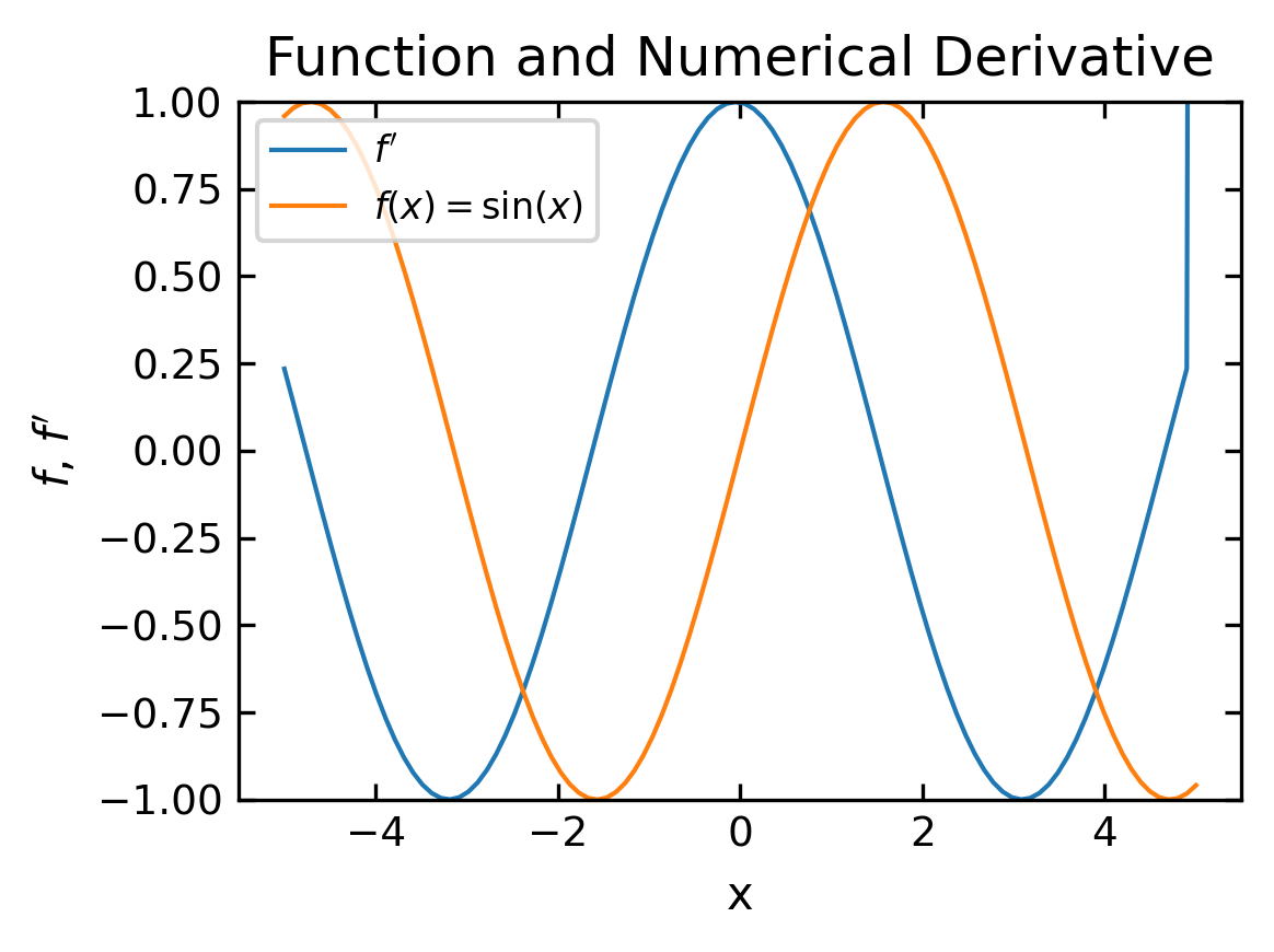
fp=m*f
[28]:
plt.figure(figsize=(4,3))
plt.plot(x[:],fp[:],label='$f^{\prime}$')
plt.plot(x,f,label='$f(x)=\sin(x)$')
plt.xlabel('x')
plt.ylabel('$f$, $f^{\prime}$')
plt.legend()
plt.ylim(-1,1)
plt.title('Function and Numerical Derivative')
plt.tight_layout()
plt.show()
Check yourself, that the following line of code will calculate the second derivative.
m=diags([-2., 1., 1.], [0,-1, 1], shape=(100, 100))