Dipole Radiation
We would like to examine the origin of electromagnetic radiation in a classical picture. Especially we would like to understand why the electromagnetic fields that are radiated are transverse to the direction of propagation. We will consider for this purpose the radiation generated by an accelerated charge.
Electric field of an accelerated charge
We will follow for the derivation of transverse electric field the basic steps of the derivation by Larmor. We consider a charge, which is initially at rest in the point \(O\) as sketched below. The charge is then accelerated for a very short period \(\Delta t\) to the point \(O'\) and reaches a final speed \(u\), which is small compared to the speed of light \(u \ll c\). The charge then moves with that speed up to a point \(O''\) for a time \(t\).
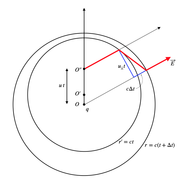
What will be important for our consideration is the fact that any information about a system’s change of state is limited in its propagation to the speed of light. Thus, the information that the charge \(q\) has been accelerated has propagated from \(O\) a distance \(r=c(t+\Delta t)\), when the charge has reached the point \(O''\). The fact that the charge stopped accelerating, which is originating from point \(O'\) has traveled a distance \(r'=ct\).
Consider now the field line of the electric field that exists outside the outer circle which would trace back to point \(O\). This field line has now moved with the charge and is inside the inner circle corresponding to the red line. This field line needs to be connected to the remaining part outside the outer circle, as it is the same field line. Thus the field line needs to bend accordingly in the shell between the circles as indicated by the red line.
The bent part of the field vector can be decomposed into a field component perpendicular (\(E_\perp\)) to the direction from \(O\) and one parallel to this radial direction (\(E_{||}\)). The perpendicular component is the new thing and we would like to calculate it.
The ratio of perpendicular and parallel component is then given by
\[ \frac{E_{\perp}}{E_{||}}=\frac{u_{\perp}t}{c\Delta t}=\frac{a_{\perp}\Delta t t }{c\Delta t} \]
where the ratio of the electric fields is the same as of the velocity components. The velocity \(u_{\perp}\) thereby follows directly from the component of the acceleration perpendicular to the radial direction \(a_{\perp}\). The result of this calculation is then independent of the time period \(\Delta t\) and we obtain
\[ E_{\perp}=\frac{a_{\perp}r}{c^2}E_{||} \]
where we replaced the time \(t\) by \(t=r/c\). To obtain \(E_{\perp}\) we now need to know the value of \(E_{\parallel}\), which we can obtain by Gauss’s theorem considering a “pillbox” around the boundary of the sphere emanating from \(O\). Since the field lines from \(O\) are radially outwards, this calculation yields
\[ E_{\perp}=-\frac{a_{\perp}}{c^2}\frac{q}{4\pi \epsilon_0 r^2}=-\frac{a_{\perp} q}{c^24\pi \epsilon_0 r} \]
This electric field that is generated is now not anymore radially pointing outwards from the source, but it is tangential to a sphere around \(O\). It further decays with the distance as \(1/r\) and not \(1/r^2\) as the common Coulomb field. The distance dependence is consistent with the one developed earlier for spherical waves. As we know that this electric field \(E_{\perp}\) is tangential to the sphere surface we may write down the radiated field of the accelerated charge as
\[ \vec{E}(\vec{r},t)=-\frac{a_{\perp}q}{c^2 4\pi \epsilon_0 r}\hat{\theta} \]
and the corresponding magnetic field as
\[ \vec{B}(\vec{r},t)=\frac{\vec{E}}{c}=-\frac{a_{\perp}q}{c^3 4\pi \epsilon_0 r}\hat{\phi} \]
where \(\hat{\theta}\) and \(\hat{\phi}\) are the unit vectors along the polar and azimuthal direction.
Note that in the above equation the electric field is observed at time \(t\) but the acceleration has happened a time \(t-\frac{r}{c}\) earlier as it propagates with finite speed. This will finally lead to our wavelike propagation.
Energy flow
With the help of the Poynting vector
\[ \vec{S}(\vec{r},t)=\frac{1}{\mu_0} \vec{E} \times \vec{B} \]
we may now have a look at the energy flow from the accelerated charge. Since the electric and the magnetic field are orthogonal we can readily obtain the magnitude of the Poynting vector
\[ S(\vec{r},t)=\frac{a_{\perp}^2 q^2}{\mu_0 c^5 (4\pi \epsilon_0)^2 r^2} \]
from which now follows with \(a_{\perp}=a\sin{\theta}\)
\[ S(\vec{r},t)=\frac{a^2 q^2\sin^2(\theta)}{\mu_0 c^5 (4\pi \epsilon_0)^2 r^2} \]
or
\[ S(\vec{r},t)=\frac{a^2 q^2\sin^2(\theta)}{c^3 (4\pi \epsilon_0)^2 r^2} \]
The total power that is then radiated by the accelerated charge is given as the integral of the Poynting vector over a closed surface around the charge, i.e.
\[ P=\int\int S dA=\frac{a^2 q^2\sin^2(\theta)}{c^3 (4\pi \epsilon_0)^2}\int_0^{2\pi}\int_{0}^{\pi}\frac{\sin^2(\theta)}{r^2}r^2 \sin(\theta) d\theta d\phi \]
which upon integration finally yields Larmor’s formula
\[ P=\frac{q^2a^2}{6\pi c^3 \epsilon_0} \]
This is the total radiated power of an accelerated charge.
Oscillating Dipole
With the previous section we are now ready to have a look at a situation where the charge is oscillating, for example, around a fixed positive charge. This situation can occur when an atom is polarized by the electric field of an incident light wave. Since this electric field is in the visible range of a wavelength much longer than the size of the atom, we may consider the atom as being in a homogeneous oscillating electric field as we did already earlier. This approximation is called the Rayleigh limit and the process is termed Rayleigh Scattering. Let’s assume the charge is oscillating at a frequency \(\omega\) such that its displacement from the positive charge is
\[ x=x_0 e^{i\omega t} \]
from which we obtain the velocity
\[ \dot{x}=ix_0 \omega e^{i\omega t} \]
and finally the required acceleration
\[ \ddot{x}=a=-x_0 \omega^{2}e^{i\omega t} \]
The product of charge and acceleration which enters the generated electric field can then be expressed as
\[ q a=-q x_{0}\omega^{2}e^{i\omega t} = -p \omega^{2}e^{i\omega t} \]
since the dipole moment is given by \(p=q x_0\). Consequently, the electric field radiated by an oscillating dipole is given by
\[ E(\vec{r},t)=-\frac{a_{\perp} q}{c^24\pi \epsilon_0 r}=\frac{p\omega^2 \sin^2(\theta)}{c^2 4\pi\epsilon_0 r}e^{i\omega t} \]
The direction of the electric and also the magnetic field can now be constructed with the appropriate unit vector in the radial direction as well as the direction of the dipole moment \(\vec{p}\). The perpendicular component of the dipole moment including its direction is given by \((\hat{e}_r\times \vec{p})\times \hat{e}_r\) such that we obtain the electric and magnetic field in its vectorial beauty
\[\begin{eqnarray} \vec{E}(\vec{r},t) & = &\frac{\omega^2}{4\pi \epsilon_0 c^2 r}(\hat{e}_r\times \vec{p})\times \hat{e}_r e^{i(k r - \omega t)}\\ \vec{B}(\vec{r},t) & = &\frac{\omega^2}{4\pi \epsilon_0 c r}(\hat{e}_r\times \vec{p}) e^{i(k r - \omega t)} \end{eqnarray}\]
This corresponds to the radiated field of an oscillating dipole at large distances (\(r \gg \lambda\)), which is called the far field. In the near field, there are additional components of the electric field which are not propagating and quickly decaying. The total electric field of an oscillating dipole is given by
\[ \vec{E}(\vec{r},t)=\frac{\omega^3}{4\pi \epsilon_0 c^3} \left [ ((\hat{e}_r\times \vec{p})\times \hat{e}_r)\frac{1}{k r}+3(\hat{e}_r(\hat{e}_r\cdot \vec{p})-\vec{p})\left(\frac{1}{(k r)^3}-\frac{i}{(kr)^2} \right)\right] e^{i(kr -i \omega t)} \]
With the help of the dipole field we thus obtain the intensity radiated by an oscillating dipole at
\[ I(\theta)=\frac{\omega^4|\vec{p}|^2}{32\pi^2 \epsilon_0 c^3}(1-\cos^2(\theta)) \]
and the radiated power is given by
\[ P=\frac{\omega^4 |\vec{p}|^2}{12\pi \epsilon_0 c^3}=\left (\frac{2\pi}{\lambda}\right )^4\frac{c|\vec{p}|^2}{12\pi \epsilon_0} \tag{radiated power of an oscillating dipole} \]
As frequencies are not as intuitive in our daily color language, we have converted that expression to contain the wavelength of light, which tells us that the power radiated scales with the inverse of the wavelength to the power of four. This means for visible light that blue light is scattered much stronger than red light.
This \(\lambda^{-4}\) dependence, known as Rayleigh scattering, explains why the sky appears blue during the day. As sunlight travels through the atmosphere, it encounters molecules much smaller than its wavelength. These molecules scatter blue light (\(\lambda \approx 450\, nm\)) about 10 times more strongly than red light (\(\lambda \approx 700\, nm\)), causing the sky’s characteristic blue color.
The same effect explains why sunsets appear red. When the Sun is near the horizon, sunlight travels through more atmosphere to reach our eyes, approximately through a path length \(L \propto 1/\cos{\theta}\), where \(\theta\) is the angle from the zenith. The increased scattering of blue light along this longer path, following \(I \propto L\lambda^{-4}\), leaves primarily red wavelengths to travel directly to the observer.
This fundamental process governs not only our sky’s appearance but can also be observed in other natural phenomena. For instance, scattered light in colloidal suspensions follows the same wavelength dependence when the scattering particles are much smaller than the wavelength of light (\(d \ll \lambda\)), creating similar color effects in smoke and certain liquids.
Interactive Visualization: Oscillating Dipole Electric Field
Below is an interactive visualization of the electric field from an oscillating dipole in the x-z plane, showing both near-field and far-field components as a color-coded heatmap.
When particles become comparable to or larger than the wavelength of light (\(d \geq \lambda\)), Rayleigh scattering no longer adequately describes the physics. In this regime, Mie scattering becomes dominant. For a dielectric sphere with relative permittivity \(\epsilon_r\), the scattered intensity can be expressed as a series solution to Maxwell’s equations:
\[I(\theta) = \frac{\lambda^2}{4\pi^2r^2}(|S_1(\theta)|^2 + |S_2(\theta)|^2)\]
where \(S_1\) and \(S_2\) are complex scattering amplitudes containing Bessel functions and Legendre polynomials. The size parameter \(x = 2\pi r/\lambda\) and the relative refractive index \(m = \sqrt{\epsilon_r}\) determine the scattering behavior. For dielectric particles, \(m\) is real, leading to primarily directive scattering. The scattering cross-section \(\sigma\) for intermediate-sized dielectric particles can be approximated as:
\[\sigma \approx \pi r^2 \left(2 - \frac{4}{x}\sin{x} + \frac{4}{x^2}(1-\cos{x})\right)\]
Modern materials engineering has extended these concepts to metamaterials, where engineered structures create effective medium properties not found in nature. For these materials, both \(\epsilon_r\) and the relative permeability \(\mu_r\) can be complex and frequency-dependent:
\[\epsilon_r(\omega) = 1 - \frac{\omega_p^2}{\omega^2 + i\gamma\omega}, \quad \mu_r(\omega) = 1 - \frac{F\omega^2}{\omega^2 - \omega_0^2 + i\gamma\omega}\]
Here, \(\omega_p\) is the plasma frequency, \(\omega_0\) the resonance frequency, and \(\gamma\) the damping factor. These materials can exhibit negative refractive indices or epsilon-near-zero behavior, leading to unusual scattering patterns and applications in perfect lenses or electromagnetic cloaking. The Mie theory has been extended to these cases by allowing complex values of \(m\), though the mathematical framework remains similar.
This generalized theory explains phenomena ranging from atmospheric optics to the design of nanophotonic devices and metamaterial-based sensors. The interaction between light and matter becomes particularly intricate when dealing with plasmonic materials or structures with engineered electromagnetic responses.