Diffraction in Applications

Application: Resolution of an Optical Microscope

The resolution of an optical microscope is fundamentally limited by the diffraction of light as it passes through the optical components, particularly the objective lens. Diffraction causes point sources of light to produce blurred images rather than perfect points, affecting the microscope’s ability to distinguish between two closely spaced objects.

Rayleigh’s Criterion for Resolution

Key Question: How close can two point sources be while still being perceived as distinct entities by an optical system?

To answer this, we need to consider two essential aspects of how a lens modifies light:

  1. Wavefront Transformation: A lens alters the curvature of incoming wavefronts, focusing parallel rays (plane waves) to a point in the focal plane.

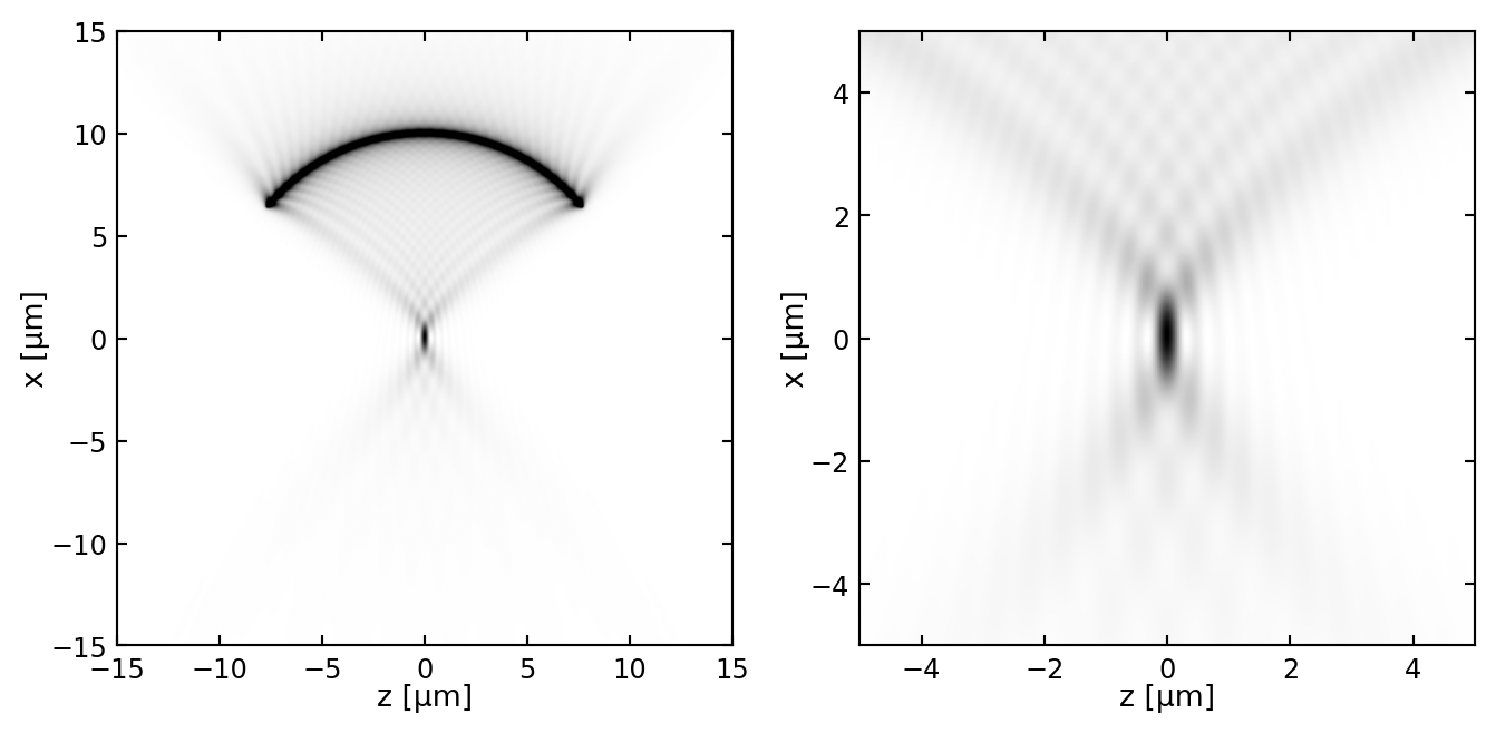
  2. Finite Aperture Effects: The lens has a finite size and acts as a circular aperture, introducing diffraction effects that spread the image of a point source into a diffraction pattern known as the Airy disk.

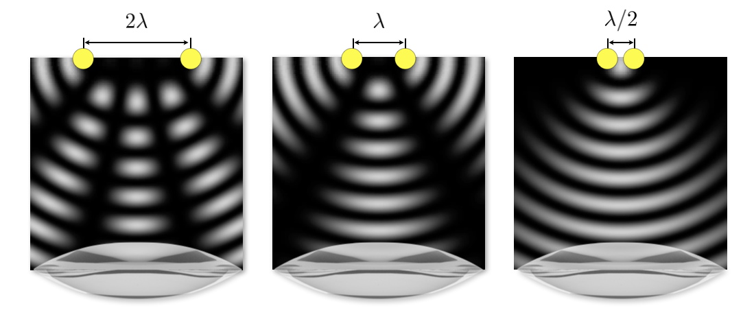
Visual Representation:

Illustration showing two point sources and their overlapping diffraction patterns as they approach each other.

Each point source produces its own diffraction pattern. As the sources move closer, their patterns begin to overlap, making it harder to distinguish between them.

Rayleigh’s Resolution Criterion:

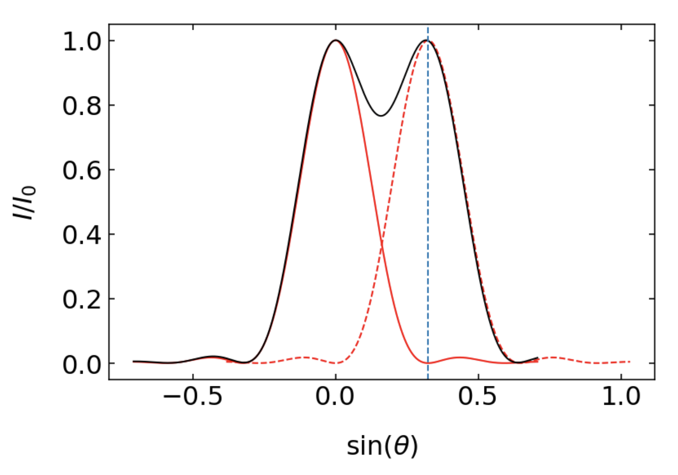
  • Two point sources are considered just resolvable when the principal maximum (center) of one Airy pattern coincides with the first minimum (dark ring) of the other.

Graph depicting Rayleigh’s criterion, showing the intensity profiles of two overlapping Airy patterns.

For incoherent light sources (where the light waves are not in phase), this criterion corresponds to a 26% dip in intensity between the two peaks, which is generally sufficient for the human eye or detectors to distinguish the two sources as separate.

Angle to the First Minimum:

The angle \(\theta_1\) to the first minimum of the diffraction pattern from a circular aperture of radius \(R\) is given by:

\[ \sin(\theta_1) = 1.22\, \frac{\lambda}{2R} \]

Since the diameter of the aperture \(D = 2R\), this can also be written as:

\[ \sin(\theta_1) = 1.22\, \frac{\lambda}{D} \]

The factor 1.22 arises from the first zero of the Bessel function \(J_1\) that describes the diffraction pattern of a circular aperture.

Small Angle Approximation:

For small angles (common in optical systems), \(\sin(\theta_1) \approx \theta_1\) in radians.

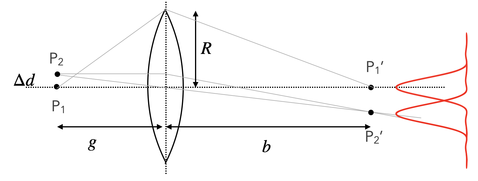
Relating Angular to Linear Separation in the Image Plane:

The angular resolution \(\theta_1\) corresponds to a linear separation \(\Delta x\) in the image plane (at image distance \(b\)):

\[ \theta_1 = \frac{\Delta x}{b} \]

Combining the Equations:

Substituting \(\theta_1\):

\[ \frac{\Delta x}{b} = 1.22\, \frac{\lambda}{D} \]

Solving for \(\Delta x\):

\[ \Delta x = 1.22\, \frac{\lambda b}{D} \]

Considering the Object Plane:

The magnification \(M\) of the optical system is:

\[ M = \frac{b}{g} \]

where \(g\) is the object distance. The corresponding separation in the object plane (\(\Delta d\)) is:

\[ \Delta d = \frac{\Delta x}{M} = \frac{\Delta x \, g}{b} \]

Substituting \(\Delta x\):

\[ \Delta d = 1.22\, \frac{\lambda b}{D} \times \frac{g}{b} = 1.22\, \frac{\lambda g}{D} \]

Introducing Numerical Aperture (NA):

The numerical aperture (NA) of the lens is defined as:

\[ \text{NA} = n \sin(\alpha) \]

where:

  • \(n\) is the refractive index of the medium between the object and the lens.
  • \(\alpha\) is the half-angle of the maximum cone of light that can enter or exit the lens.

Since \(\sin(\alpha) = \frac{R}{g}\), we have:

\[ D = 2R = 2 g \sin(\alpha) \]

Substituting \(D\) into \(\Delta d\):

\[ \Delta d = 1.22\, \frac{\lambda g}{2 g \sin(\alpha)} = \frac{1.22\, \lambda}{2 \sin(\alpha)} = \frac{0.61\, \lambda}{\sin(\alpha)} \]

Therefore, incorporating the refractive index \(n\):

\[ \Delta d = \frac{0.61\, \lambda}{n \sin(\alpha)} = \frac{0.61\, \lambda}{\text{NA}} \]

Under Rayleigh’s resolution criterion, several key factors influence the resolving power of an optical system.

Firstly, a higher numerical aperture (NA) improves resolution. This increase can be achieved by enhancing either the refractive index \(n\) of the medium between the object and the lens or the sine of the collection angle \(\sin(\alpha)\). Since the NA is defined as \(\text{NA} = n \sin(\alpha)\), a larger NA allows the lens to gather more diffracted light, thereby resolving finer details in the image. In air, where the refractive index is approximately \(n \approx 1\), the maximum achievable NA is less than 1, which limits the resolution. This limitation arises because the maximum value of \(\sin(\alpha)\) is 1 (when \(\alpha = 90^\circ\)), so the NA in air cannot exceed 1. In practical systems, the collection angle \(\alpha\) is much less than \(90^\circ\), further reducing the NA and thus the resolution. Immersion lenses, which use a medium with a higher refractive index (such as water or oil), can achieve higher NAs, overcoming this limitation and improving resolution.

Secondly, using shorter wavelengths \((\lambda)\) of light leads to better resolution. According to the formula \(\Delta d = \frac{0.61\, \lambda}{\text{NA}}\), the minimum resolvable distance \(\Delta d\) is directly proportional to the wavelength. Therefore, decreasing the wavelength reduces \(\Delta d\), allowing the optical system to distinguish smaller features of the object.

Rayleigh’s Resolution Criterion

Two incoherent point sources can be resolved when their minimum separation \(\Delta d\) satisfies:

\[ \Delta d \geq \frac{0.61\, \lambda}{\text{NA}} \]

Here \(\Delta d\) is the minimum resolvable distance between the two point sources, \(\lambda\) is the wavelength of the light used for imaging, and \(\text{NA} = n \sin(\alpha)\) is the numerical aperture of the optical system, where \(n\) is the refractive index of the medium and \(\alpha\) is the half-angle of the maximum cone of light entering the lens.

Abbe’s Criterion for Resolution

While Rayleigh’s criterion applies to incoherent light sources where intensities add directly, Ernst Abbe developed a complementary theory for coherent imaging in the context of microscopy. Abbe’s approach emphasizes the role of diffracted orders and spatial frequencies in image formation.

Abbe recognized that an object with fine periodic details acts as a diffraction grating, scattering incident coherent light into multiple diffraction orders: the zeroth order (undiffracted beam), and higher orders (±1st, ±2nd, etc.). Each order carries information about different spatial frequency components of the object. For the optical system to correctly reproduce the image, it must capture at least the zeroth order and one first-order beam. If the objective lens aperture is too small and blocks all first-order diffracted beams, the fine structural details cannot be resolved regardless of magnification.

Consider a periodic structure with spacing \(d\). When illuminated with coherent light of wavelength \(\lambda\), the first diffraction order emerges at angle \(\theta\) satisfying the grating equation \(d \sin\theta = \lambda\). For the objective lens to capture this first order, we require \(\sin\theta \leq \sin\alpha\), where \(\alpha\) is the half-angle of the cone of light accepted by the lens. The smallest resolvable spacing occurs when the first-order beam just enters the lens at its maximum acceptance angle:

\[ d \sin\alpha = \lambda \]

Since the numerical aperture is \(\text{NA} = n \sin\alpha\) (where \(n\) is the refractive index), this gives:

\[ \Delta d = \frac{\lambda}{n \sin\alpha} = \frac{\lambda}{\text{NA}} \]

In practical microscopy with oblique illumination or with both transmitted and reflected light beams entering from opposite sides of the optical axis, diffracted orders from both sides can enter the objective. This effectively doubles the range of spatial frequencies captured, improving the resolution by a factor of 2:

\[ \Delta d = \frac{\lambda}{2 \,\text{NA}} \]

Interference patterns demonstrating Abbe’s criterion, showing how diffraction orders combine to resolve structures at different spacings: \(\lambda\), \(\lambda\), and \(\lambda/2\) distances.
Abbe’s Resolution Criterion

According to Abbe’s theory, the minimum resolvable spacing \(\Delta d\) of a periodic object in a microscope is:

\[ \Delta d = \frac{\lambda}{2 \,\text{NA}} \]

where \(\lambda\) is the wavelength of light and \(\text{NA}\) is the numerical aperture of the objective lens. This criterion requires that the objective lens captures at least the zeroth-order and one first-order diffracted beam to resolve the periodic structure. The factor of 2 assumes optimal illumination conditions where diffracted orders from both sides of the optical axis can contribute to image formation.

Comparing Rayleigh’s and Abbe’s Criteria

The two criteria approach resolution from different physical perspectives. Rayleigh’s criterion (\(\Delta d = 0.61\lambda/\text{NA}\)) describes when two incoherent point sources become distinguishable based on the overlap of their Airy diffraction patterns, with the factor 0.61 arising from the first zero of the Bessel function \(J_1\). This applies naturally to conventional bright-field microscopy and fluorescence imaging where sources emit independently.

Abbe’s criterion (\(\Delta d = \lambda/(2\text{NA})\)) describes the spatial frequency bandwidth of an optical system for coherent imaging. It requires capturing at least two diffraction orders (zeroth and first) to resolve periodic structures. This framework applies to phase-contrast microscopy, interference microscopy, and other coherent imaging techniques.

Despite their different origins, both criteria reveal the same fundamental scaling: resolution improves linearly with numerical aperture and inversely with wavelength. The numerical factor difference (\(0.61 \approx 1.22/2\) versus \(1/2\)) reflects the different physical scenarios—intensity overlap for incoherent sources versus spatial frequency transmission for coherent illumination. Both confirm that diffraction fundamentally limits optical resolution at \(\Delta d \sim \lambda/\text{NA}\).

Application: Diffraction in the Human Eye

The human eye provides an excellent real-world example of circular aperture diffraction through the pupil (the opening in the iris). By examining how light diffracts as it enters the eye, we can understand fundamental limits on visual resolution and how the eye is naturally optimized to these constraints.

Calculating the Diffraction Limit of the Eye

When light passes through the circular aperture of the pupil, it undergoes diffraction, producing an Airy disk pattern on the retina. The angle to the first minimum (dark ring) of the diffraction pattern is given by:

\[ \sin(\theta_1) = 0.61\, \frac{\lambda}{R} \]

where:

  • \(\theta_1\) is the angle to the first minimum,
  • \(\lambda\) is the wavelength of the light,
  • \(R\) is the radius of the aperture (pupil).

For an average pupil radius of \(R = 2.5\, \text{mm}\) and green light with a wavelength of \(\lambda = 532\, \text{nm}\) (to which the human eye is most sensitive), we have:

\[ \sin(\theta_1) = 0.61 \times \frac{532 \times 10^{-9}\, \text{m}}{2.5 \times 10^{-3}\, \text{m}} = 0.61 \times 2.128 \times 10^{-4} \approx 1.298 \times 10^{-4} \]

Thus, the angle to the first minimum is approximately:

\[ \theta_1 \approx \sin^{-1}(1.298 \times 10^{-4}) \approx 0.00744^\circ \]

Determining the Size of the Airy Disk on the Retina

The distance from the pupil to the retina (the image plane) is approximately \(L = 20\, \text{mm}\) (or \(2\, \text{cm}\)). The linear radius \(r\) of the Airy disk on the retina is calculated by:

\[ r = L \sin(\theta_1) = 20\, \text{mm} \times 1.298 \times 10^{-4} = 2.596 \times 10^{-3}\, \text{mm} = 2.596\, \mu\text{m} \]

So, the diameter \(D\) of the Airy disk (central bright spot) is:

\[ D = 2r = 2 \times 2.596\, \mu\text{m} = 5.192\, \mu\text{m} \]

This means that the smallest spot of light that can be formed on the retina due to diffraction is about \(5.19\, \mu\text{m}\) in diameter.

Comparing with Photoreceptor Spacing in the Fovea

The fovea is a small region in the retina responsible for sharp central vision. It contains a high density of cone photoreceptor cells. The average density of cones in the fovea is approximately \(150,000\) cells per square millimeter. To find the average spacing \(d\) between these cells, we proceed as follows:

Area per Cell:

\[ \text{Area per cell} = \frac{1\, \text{mm}^2}{150,000} = 6.667 \times 10^{-6}\, \text{mm}^2 = 6.667\, \mu\text{m}^2 \]

Linear Spacing Between Cells:

Assuming a square packing (for simplicity), the linear spacing \(d\) is:

\[ d = \sqrt{\text{Area per cell}} = \sqrt{6.667\, \mu\text{m}^2} \approx 2.58\, \mu\text{m} \]

In reality, the photoreceptors are more closely packed in a hexagonal arrangement, but this calculation gives a good approximation.

Our calculations show that the Airy disk diameter is approximately \(5.2\, \mu\text{m}\), while the photoreceptor spacing in the fovea is about \(2.6\, \mu\text{m}\). The Airy disk thus spans roughly two photoreceptors, revealing a remarkable match between optical and biological scales.

Why the Eye’s Design is Optimal

The diffraction limit sets the fundamental constraint. Due to the wave nature of light passing through the pupil aperture, no amount of optical refinement can produce a sharper image than the Airy disk pattern. This diffraction limit determines the finest detail the eye’s optics can deliver to the retina.

The photoreceptor density is matched to this limit. With spacing of approximately \(2.6\, \mu\text{m}\), photoreceptors are dense enough to sample the detail present in the optical image. According to the Nyquist sampling theorem, you need at least two samples per feature to faithfully capture it—and that’s exactly what we find here.

Adding more photoreceptors would not improve resolution. Two factors prevent this:

  1. Physical limit: The optical system cannot resolve details finer than the Airy disk size, regardless of how many photoreceptors are present. Packing more receptors into the same area would simply record the same blurred information multiple times.

  2. Signal considerations: Each photoreceptor would receive less light (since the total light is fixed), potentially worsening the signal-to-noise ratio and making detection more difficult.

Biological Optimization

The human eye exemplifies evolutionary optimization. The photoreceptor density is precisely tuned to extract the maximum information provided by the eye’s optics, without wasteful over-sampling. This alignment between optical physics and retinal anatomy reflects millions of years of natural selection, where biological structures have been shaped to work efficiently within the constraints imposed by the laws of physics. The result is a visual system that achieves excellent performance while using biological resources efficiently—neither under-sampling (which would waste optical resolution) nor over-sampling (which would waste neural tissue and energy).

References:

  • Land, M. F., & Nilsson, D.-E. (2012). Animal Eyes (2nd ed.). Oxford University Press.
  • Williams, D. R. (1988). Topography of the foveal cone mosaic in the living human eye. Vision Research, 28(3), 433–454.

Using Huygens Sources for more

The Huygens principle is a powerful tool to calculate the diffraction pattern of an aperture. The idea is to consider the aperture as a collection of point sources, which emit spherical waves. The superposition of all these waves will then give the total wave field. Below is a Python code which demonstrates the calculation of the diffraction pattern of a spherical mirror. It uses Huygens sources placed on an arc (see left). The right image shows the resulting diffraction pattern in the focal plane of the mirror.

Code
import numpy as np
import matplotlib.pyplot as plt

def spherical_wave(k, omega, r, r0, t):
    k_norm = np.linalg.norm(k)
    d = np.linalg.norm(r - r0[:, np.newaxis, np.newaxis], axis=0)
    return np.exp(1j * (k_norm * d - omega * t)) / d

# Parameters
wavelength = 532e-9  # Wavelength in meters (green light)
k0 = 2 * np.pi / wavelength  # Wave number
c = 299792458  # Speed of light in m/s
omega0 = k0 * c  # Angular frequency
t = 0  # Time

x = np.linspace(-15e-6, 15e-6, 900)  # x-axis from -5 µm to 5 µm
z = np.linspace(-15e-6, 15e-6, 900)  # z-axis from -5 µm to 5 µm
X, Z = np.meshgrid(x, z)
r = np.array([X, np.zeros_like(X), Z])  # Observation points in 3D space (y=0)

num_sources = 100  # Number of point sources along the arc
arc_angle = np.deg2rad(100)  # Total arc angle in radians (60 degrees)
theta_sources = np.linspace(-arc_angle / 2, arc_angle / 2, num_sources)  # Source angles
radius = 10e-6  # Radius of the arc (10 µm)

total_field = np.zeros_like(X, dtype=complex)

for theta in theta_sources:
    # Calculate source position (x0, z0) on the arc
    x0 = radius * np.cos(theta)
    z0 = radius * np.sin(theta)
    r0 = np.array([x0, 0, z0])  # Source position in 3D space
    field = spherical_wave(k0, omega0, r, r0, t)
    total_field += field

intensity = np.abs(total_field)**2

intensity/=intensity[450,450]
fig,ax=plt.subplots(1,2,figsize=get_size(18, 10))

extent = [np.min(z)*1e6, np.max(z)*1e6, np.min(x)*1e6, np.max(x)*1e6]
ax[1].imshow(intensity.transpose(), extent=extent, origin='lower', cmap='gray_r',vmax=1)
ax[1].set_xlabel('z [µm]')
ax[1].set_ylabel('x [µm]')
ax[1].set_xlim(-5, 5)
ax[1].set_ylim(-5, 5)

extent = [np.min(z)*1e6, np.max(z)*1e6, np.min(x)*1e6, np.max(x)*1e6]
ax[0].imshow(intensity.transpose(), extent=extent, origin='lower', cmap='gray_r',vmax=1)
ax[0].set_xlabel('z [µm]')
ax[0].set_ylabel('x [µm]')
ax[0].set_xlim(-15, 15)
ax[0].set_ylim(-15, 15)
plt.tight_layout()
plt.show()

The pattern changes with increasing angle of the arc, which is consistent with our knowledge of the numerical aperature defining the resolution of and optical system. The changes are especially visible along the vertical axis.

Code
import numpy as np
import matplotlib.pyplot as plt

def spherical_wave(k, omega, r, r0, t):
    k_norm = np.linalg.norm(k)
    d = np.linalg.norm(r - r0[:, np.newaxis, np.newaxis], axis=0)
    return np.exp(1j * (k_norm * d - omega * t)) / d

# Parameters
wavelength = 532e-9  # Wavelength in meters (green light)
k0 = 2 * np.pi / wavelength  # Wave number
c = 299792458  # Speed of light in m/s
omega0 = k0 * c  # Angular frequency
t = 0  # Time

x = np.linspace(-15e-6, 15e-6, 900)  # x-axis from -5 µm to 5 µm
z = np.linspace(-15e-6, 15e-6, 900)  # z-axis from -5 µm to 5 µm
X, Z = np.meshgrid(x, z)
r = np.array([X, np.zeros_like(X), Z])  # Observation points in 3D space (y=0)

num_sources = 100  # Number of point sources along the arc
arc_angle = np.deg2rad(150)  # Total arc angle in radians (60 degrees)
theta_sources = np.linspace(-arc_angle / 2, arc_angle / 2, num_sources)  # Source angles
radius = 10e-6  # Radius of the arc (10 µm)

total_field = np.zeros_like(X, dtype=complex)

for theta in theta_sources:
    # Calculate source position (x0, z0) on the arc
    x0 = radius * np.cos(theta)
    z0 = radius * np.sin(theta)
    r0 = np.array([x0, 0, z0])  # Source position in 3D space
    field = spherical_wave(k0, omega0, r, r0, t)
    total_field += field

intensity = np.abs(total_field)**2

intensity/=intensity[450,450]
fig,ax=plt.subplots(1,2,figsize=get_size(18, 10))

extent = [np.min(z)*1e6, np.max(z)*1e6, np.min(x)*1e6, np.max(x)*1e6]
ax[1].imshow(intensity.transpose(), extent=extent, origin='lower', cmap='gray_r',vmax=1)
ax[1].set_xlabel('z [µm]')
ax[1].set_ylabel('x [µm]')
ax[1].set_xlim(-5, 5)
ax[1].set_ylim(-5, 5)

extent = [np.min(z)*1e6, np.max(z)*1e6, np.min(x)*1e6, np.max(x)*1e6]
ax[0].imshow(intensity.transpose(), extent=extent, origin='lower', cmap='gray_r',vmax=1)
ax[0].set_xlabel('z [µm]')
ax[0].set_ylabel('x [µm]')
ax[0].set_xlim(-15, 15)
ax[0].set_ylim(-15, 15)
plt.tight_layout()
plt.show()