Optical Elements Part III

Lenses

The most important optical elements are lenses, which come in many different flavors. They consist of curved surfaces, which most commonly have the shape of a part of a spherical cap. It is, therefore, useful to have a look at the refraction at spherical surfaces.

Refraction at spherical surfaces

For our calculations of the refraction at spherical surfaces, we consider the sketch below.

Figure 1: Refraction at a curved surface.

To derive an imaging equation for a lens, we aim to calculate the distance \(b\) and angle \(\theta_2\) at which a ray crosses the optical axis, given its origin at distance \(a\) and angle \(\theta_1\). We begin with Snell’s law for the geometry:

\[n_{1}\sin(\alpha+\theta_1)=n_{2}\sin(\alpha-\theta_2)\]

We define key relationships:

\[\sin(\alpha)=\frac{y}{R}, \quad \tan(\theta_1)=\frac{y}{a}, \quad \tan(\theta_2)=\frac{y}{b}\]

To simplify this, we employ the paraxial approximation, which assumes all angles are small. This allows us to use first-order approximations of trigonometric functions, effectively linearizing them:

\[\sin(\theta) \approx \theta+ O(\theta^{3}), \quad \tan(\theta) \approx \theta + O(\theta^{3}),\quad \cos(\theta)\approx 1 + O(\theta^{2})\]

This approach, common in optics, significantly simplifies our calculations while maintaining accuracy for most practical scenarios involving lenses.

With the help of these approximations we can write Snell’s law for the curved surface as

\[n_1(\alpha+\theta_1)=n_2(\alpha-\theta_2).\]

With some slight transformation which you will find in the video of the online lecture we obtain, therefore,

\[\theta_2=\frac{n_2-n_1}{n_2 R}y -\frac{n_1}{n_2}\theta_1,\]

which is a purely linear equation in \(y\) and \(\theta_1\).

Paraxial Approximation

The paraxial approximation is a fundamental simplification in optics that assumes all angles are small. This allows us to use linear approximations for trigonometric functions, significantly simplifying calculations while maintaining accuracy for most practical scenarios involving lenses.

To visualize the validity of this approximation, let’s examine two plots:

The first plot compares sin(θ) (blue line) with its linear approximation θ (red dashed line) for angles ranging from 0 to π/2 radians.
The second plot shows the absolute error between sin(θ) and θ.

These plots demonstrate that:

For small angles (roughly up to 0.5 radians or about 30 degrees), the approximation is very close to the actual sine function.
The error increases rapidly for larger angles, indicating the limitations of the paraxial approximation.

In most optical systems, especially those involving lenses, the angles of incident and refracted rays are typically small enough for this approximation to be valid. However, it’s important to be aware of its limitations when dealing with wide-angle optical systems or scenarios where precision is critical.

Code

import numpy as np
import matplotlib.pyplot as plt
# Define the range of angles (in radians)
theta = np.linspace(0, np.pi/2, 1000)

# Calculate sin(theta) and theta (linear approximation)
sin_theta = np.sin(theta)
linear_approx = theta

# Calculate the absolute error
error = np.abs(sin_theta - linear_approx)

# Create the plot with two subplots side by side
fig, (ax1, ax2) = plt.subplots(1, 2, figsize=(7.5, 4))

# Plot sin(theta) and theta on the first subplot
ax1.plot(theta, sin_theta, label='sin(θ)', color='blue')
ax1.plot(theta, linear_approx, label='θ', color='red', linestyle='--')
ax1.set_xlabel(r'$\theta$ [rad]')
ax1.set_ylabel(r'$\sin(x),x$')
ax1.legend()

# Plot the error on the second subplot
ax2.plot(theta, error, label='Absolute Error', color='green')
ax2.set_xlabel(r'$\theta$ [rad]')
ax2.set_ylabel('|sin(θ) - θ|')
ax2.legend()

# Adjust the layout and display the plot
plt.tight_layout()
plt.show()

Visualization of the paraxial approximation plotting the \(\sin(\theta)\) and the linear approximation \(\theta\) (dashed line) for angles ranging from 0 to \(\pi/2\) radians.

Consider light originating from a point at distance \(y\) from the optical axis. We’ll analyze two rays: one traveling parallel to the optical axis and hitting the spherical surface at height \(y\), and another incident at \(y=0\).

Figure 2: Image formation at a curved surface.

Applying our derived formula to these two cases:

For the parallel ray (\(\theta_1=0\)):

\[\theta_2=\frac{n_2-n_1}{n_2}\frac{y}{R}\] \[\theta_2=\frac{y+\Delta y}{b}\]

Equating these expressions:

\[\frac{y+\Delta y}{b}=\frac{n_2-n_1}{n_2}\frac{y}{R}\]

For the ray through the center (\(y=0\)):

\[n_2\frac{\Delta y}{b}=n_1\frac{y}{a}\]

Combining these equations yields the imaging equation for a curved surface:

\[\frac{n_1}{a}+\frac{n_2}{b}=\frac{n_2-n_1}{R}\]

We can define a new quantity, the focal length, which depends only on the properties of the curved surface:

\[f=\frac{n_2}{n_2-n_1}R\]

Imaging Equation for Spherical Refracting Surface

The sum of the inverse object and image distances equals the inverse focal length of the spherical refracting surface:

\[\frac{n_1}{a}+\frac{n_2}{b}\approx\frac{n_2}{f}\]

where the focal length of the refracting surface is given by:

\[f=\frac{n_2}{n_2-n_1}R\]

in the paraxial approximation.

Thin lens

In our previous calculation we have found a linear relation between the incident angle \(\theta_1\) with the optical axis, the incident height of the ray \(y\) and the outgoing angle \(\theta_2\):

Analyzing refraction in a lens involves two spherical surfaces. Light initially travels from a medium with refractive index \(n_1\) into the lens material with index \(n_2\). The first surface’s radius, \(R_1\), is typically positive for a convex surface facing the incident light.

At the second surface, the outgoing angle from the first refraction becomes the incident angle for the second refraction. Here, light travels from \(n_2\) back into \(n_1\). The radius \(R_2\) of this surface often has a negative value in a converging lens due to its opposite curvature relative to the optical axis.

Figure 3: Refraction on two spherical surfaces.

For thin lenses, where the thickness \(d\) is much smaller than \(R_1\) and \(R_2\) (\(d \ll R_1, R_2\)), we can simplify our analysis. We assume that the height of the ray at both surfaces is approximately equal (\(y \approx y'\)), neglecting the displacement inside the lens.

This simplification allows us to treat all refraction as occurring on a single plane at the lens center, known as the principal plane. This concept, illustrated by the dashed line in the figure, greatly simplifies optical calculations and ray tracing for thin lenses.

The radii’s sign convention (positive for convex surfaces facing incident light, negative for concave) and this two-surface analysis form the basis for the thin lens formula. This formula relates object distance, image distance, and focal length, encapsulating the lens’s imaging properties.

The result of the above calculation is leading to the imaging equation for the thin lens.

Imaging Equation for Thin Lens

The sum of the inverse object and image distances equals the inverse focal length of the thin lens:

\[\frac{1}{a}+\frac{1}{b}\approx\frac{n_2-n_1}{n_1}\left (\frac{1}{R_1}-\frac{1}{R_2}\right )=\frac{1}{f}\]

Lensmaker equation

The focal length of a thin lens is calculated by the lensmaker equation: \[f=\frac{n_1}{n_2-n_1}\left ( \frac{R_1 R_2}{R_2 -R_1}\right)\]

in the paraxial approximation.

The equation for the focal length has some important consequence. It says that if the difference of the refractive indices inside (\(n_2\)) and outside \(n_1\) get smaller, the focal length becomes larger and finally infinity. This can be nicely observed by placing a lens outside and inside a water filled basin as shown below.

Bessel’s method to measure the focal length of a lens

The is an interesting way to measure the focal length of a lens. Fix a distance \(D\) between object and screen. Then place a converging lens between them. Due to the reversibility of the light path, the lens will create a sharp image on the screen at two positions, which are separated by a distance \(d\).

The equation for the focal distance can then be obtained from the

Lens equation: \(\frac{1}{f} = \frac{1}{a} + \frac{1}{b}\)
Total distance: \(D = a + b\)

Where \(f\) is focal length, \(a\) is object distance, and \(b\) is image distance. To obtain the focal distance according to this method, which is called the Bessel method, the following steps are taken:

For the first lens position:

\[D = a_1 + b_1\]

For the second lens position:

\[D = a_2 + b_2\]

We can further calculate the distance between the two lens positions:

\[d = a_1 - a_2 = b_2 - b_1\]

and use the imaging equation to find the focal length:

\[\frac{1}{f} = \frac{1}{a_1} + \frac{1}{b_1} = \frac{1}{a_2} + \frac{1}{b_2}\]

Substituting \(b_1 = D - a_1\) and \(b_2 = D - a_2\) we get further

\[\frac{1}{f} = \frac{1}{a_1} + \frac{1}{D-a_1} = \frac{1}{a_2} + \frac{1}{D-a_2}\]

Both euqations can be solved by

\[a_1 = \frac{D + d}{2} \quad \text{and} \quad a_2 = \frac{D - d}{2}\]

If we substitute that back into the imaging equation we obtain

\[\frac{1}{f} = \frac{2}{D} + \frac{2}{d}\]

which can be rearranged to get Bessel’s formula:

\[f = \frac{D^2 - d^2}{4D}\]

This method only requires measuring \(D\) (fixed distance) and \(d\) (distance between lens positions). It eliminates the need to know exact object or image distances from the lens, making it more accurate than methods requiring precise distance measurements from the lens.

Image Construction

Images of objects can be now constructed if we refer to rays which do not emerge from a position on the optical axis only. In this case, we consider three different rays (two are actually enough). If we use as in the case of a concave mirror a central and a parallel ray, we will find a position where all rays cross on the other side. The conversion of the rays is exactly the same as in the case of a spherical mirror. The relation between the position of the object and the image along the optical axis is described by the imaging equation.

Similar to the concave mirror, we may now also find out the image size or the magnification of the lens.

Magnification of a Lens

The magnification is given by:

\[M=\frac{h_{\rm image}}{h_{\rm object}}=-\frac{b}{a}=\frac{f}{f-a}\]

where the negative sign is the result of the reverse orientation of the real images created by a lens.

According to our previous consideration \(M<0\) corresponds to a reversed image, while it is upright as the object for \(M>0\). We, therefore, easily see the following:

Object Position	Image Characteristics	Magnification (M)	Image Type
\(a < f\)	Upright and magnified	\(M > 0\)	Virtual
\(f < a < 2f\)	Reversed and magnified	\(M < -1\)	Real
\(a = 2f\)	Reversed, same size	\(M = -1\)	Real
\(a > 2f\)	Reversed and shrunk	\(-1 < M < 0\)	Real
\(a = f\)	Appears at infinity	\(M = \infty\)	-

The image below illustrates the construction of images in 4 of the above cases for a bi-convex lens, including the generation of a virtual image.


Fig.: Image construction on a biconvex lens with a parallel and a central ray for different object distances.

Thick lens

For a thin lens, the displacement of the beam in height (\(y,y^{\prime}\)) due to the thickness has been neglected. That means that we can reduce all refracting action of the lens to a single plane, which we call a principle plane. This approximation is (independent of the paraxial approximation) not anymore true for lenses if the displacement \(\Delta\) of the ray as in the image below cannot be neglected. Such lenses are called thick lenses and they do not have a single principle plane anymore. In fact, the principle plane splits up into two principle planes at a distance \(h\).

As indicated in the sketch above, an incident ray which is not deflected can be extended to its intersection with the optical axis at a point, which is a distance \(h_1\) behind the lens surface. This is the location for the first principle plane. The position of the second principle plane at a distance \(h_2\) before the back surface is found for by reversing the ray path. According to that, both principle planes have a distance \(h=d-h_1+h_2\) (mind the sign of the \(h\)). Using some mathematical effort, one can show that the same imaging equation as for a thins lens can be used with a new definition of the focal length and taking into account that object and image distances refer to their principle planes.

Matrix Optics

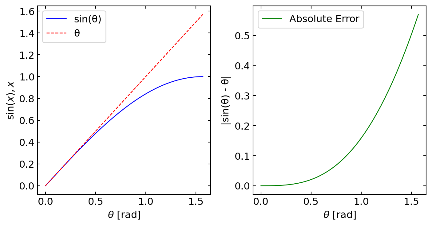
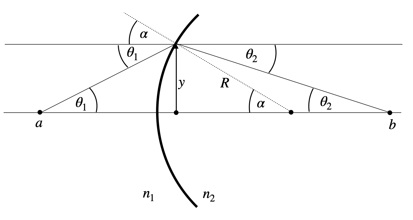
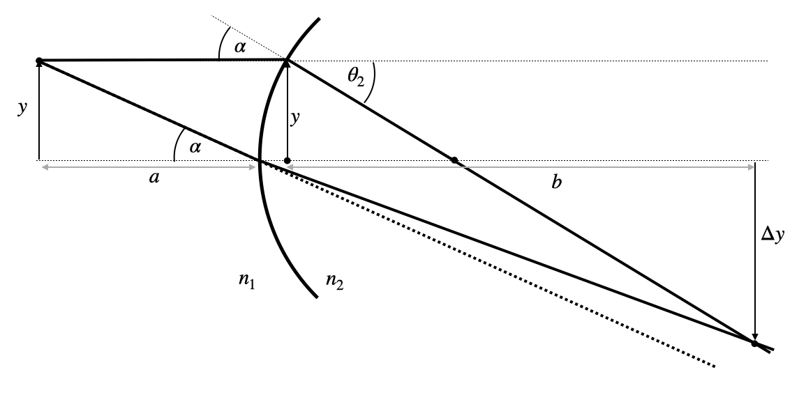
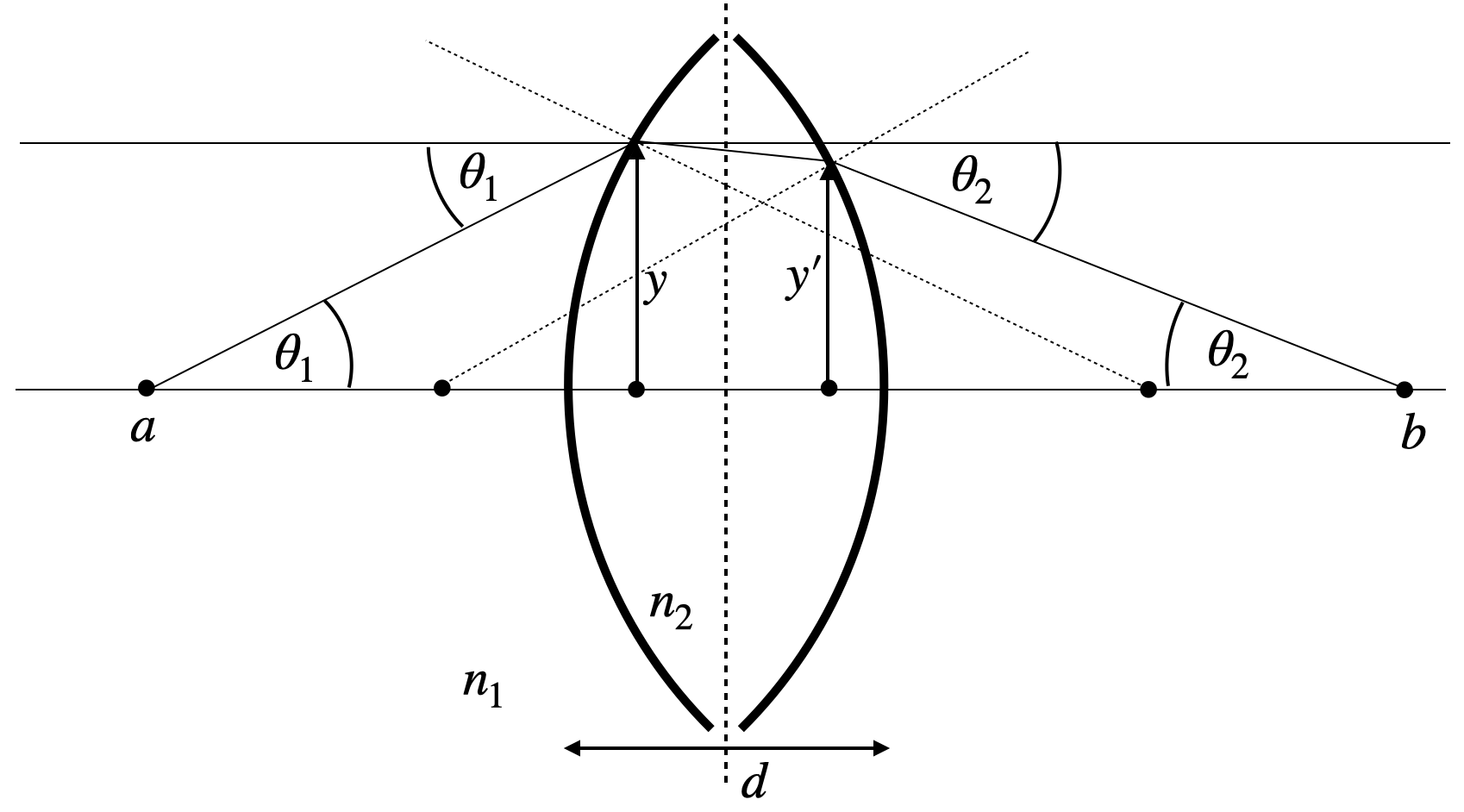
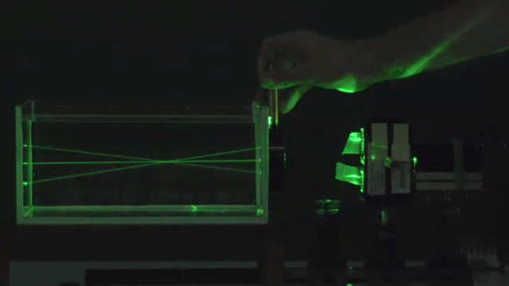
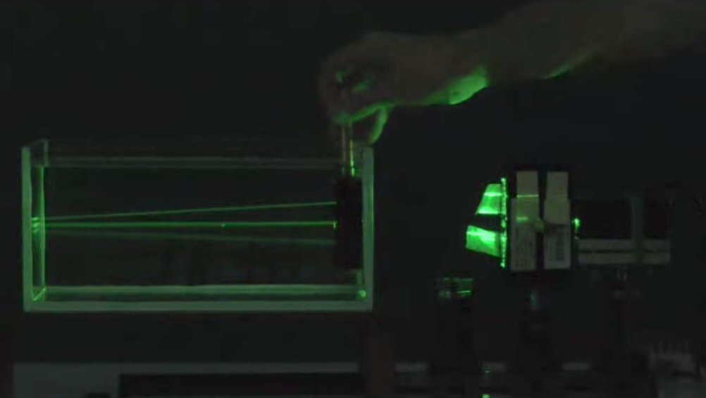
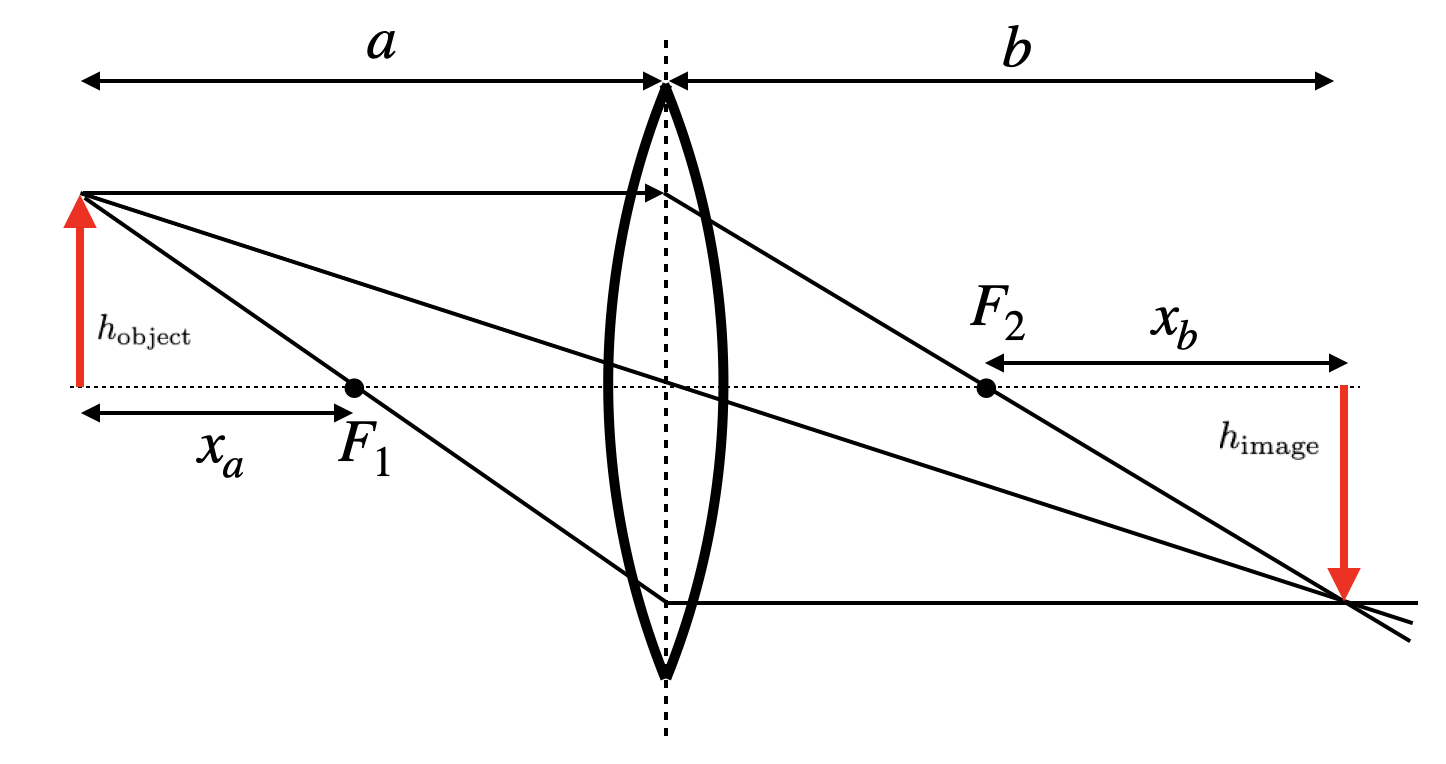
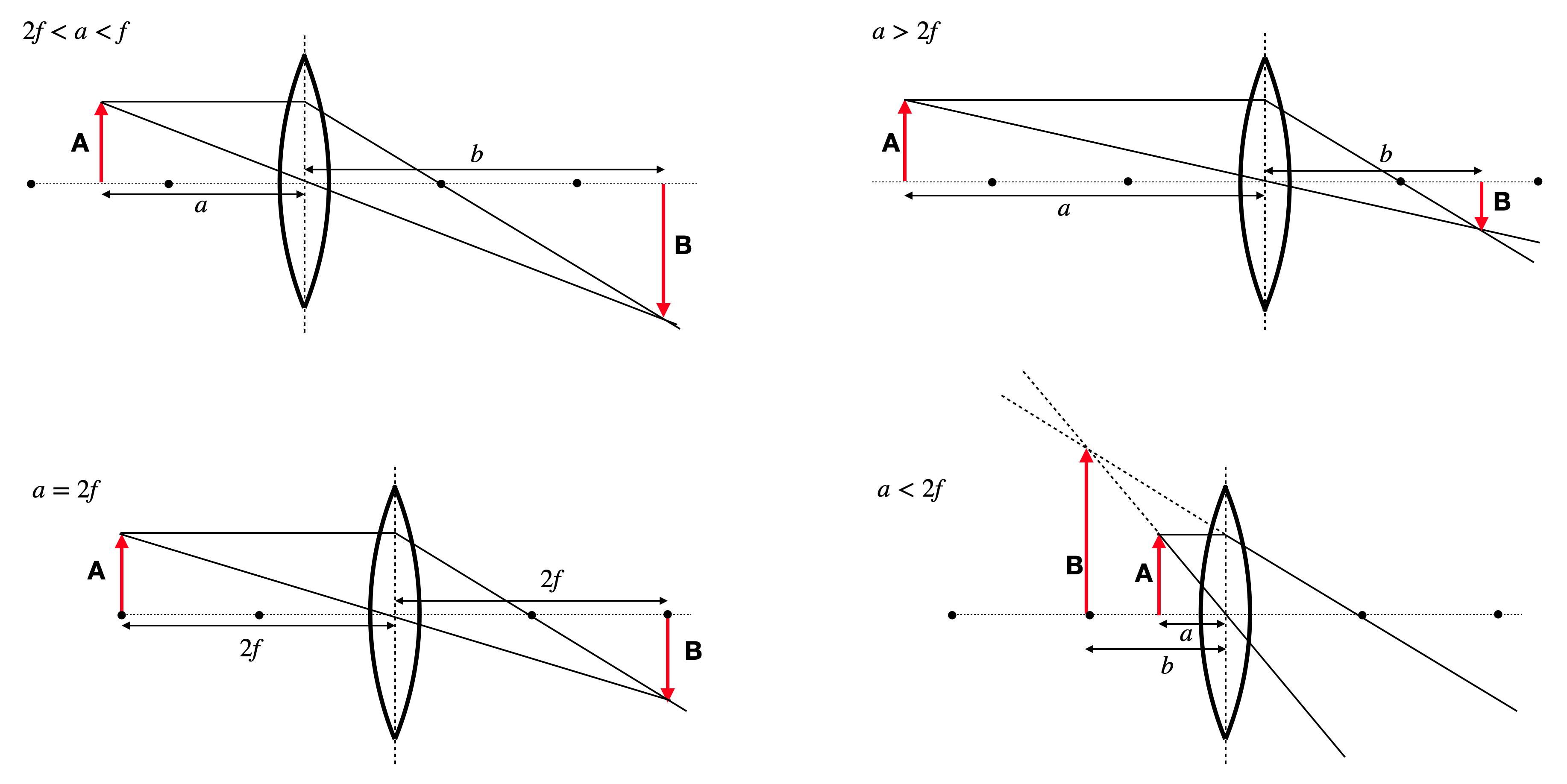
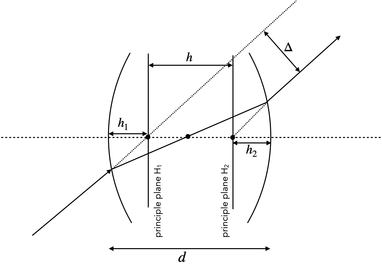
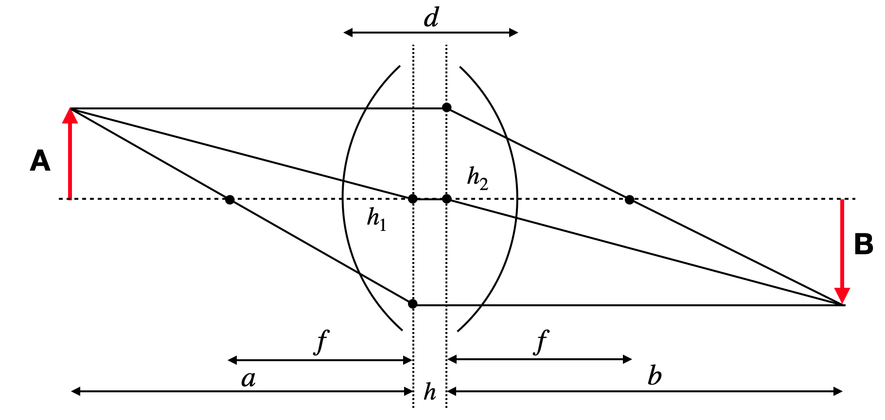
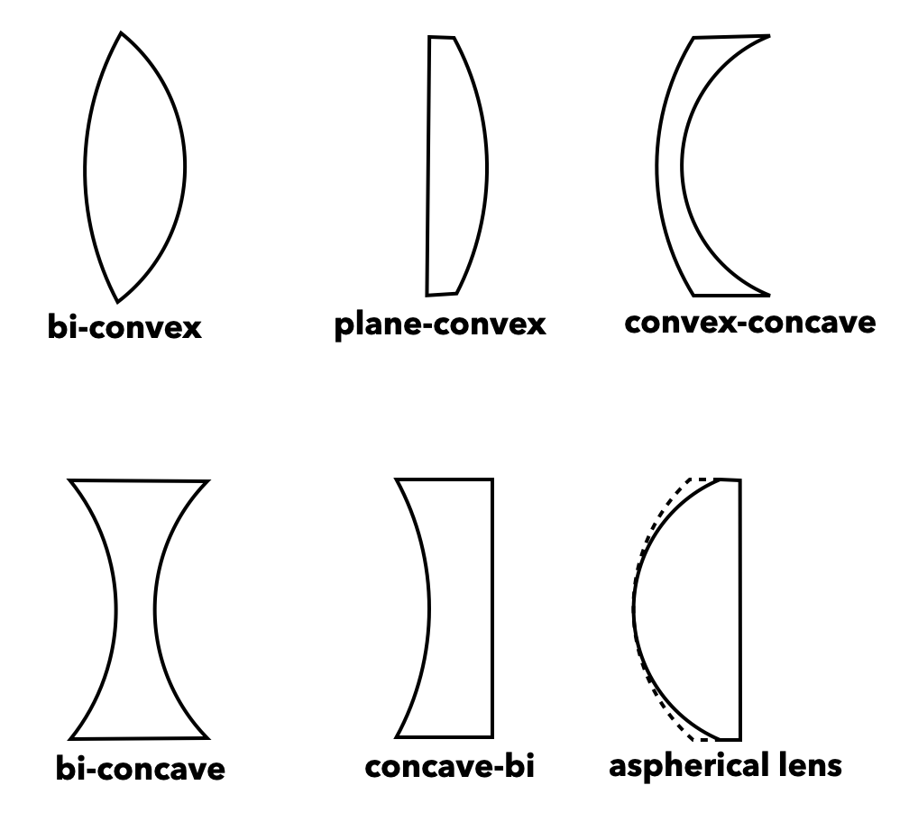
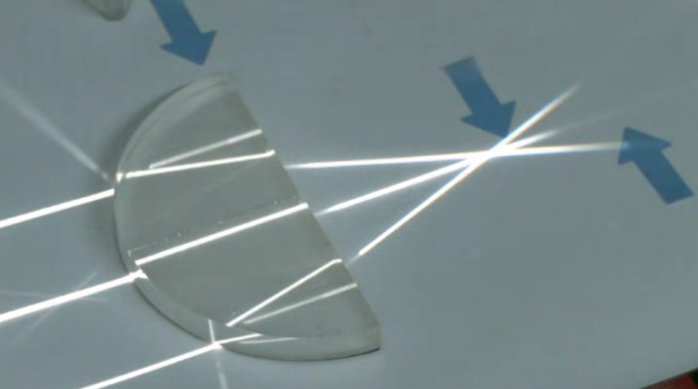
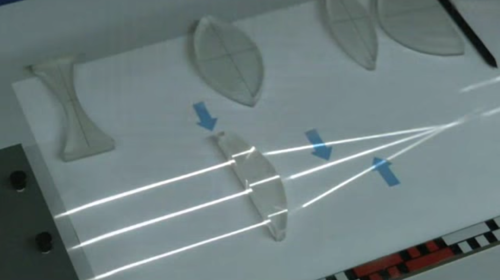
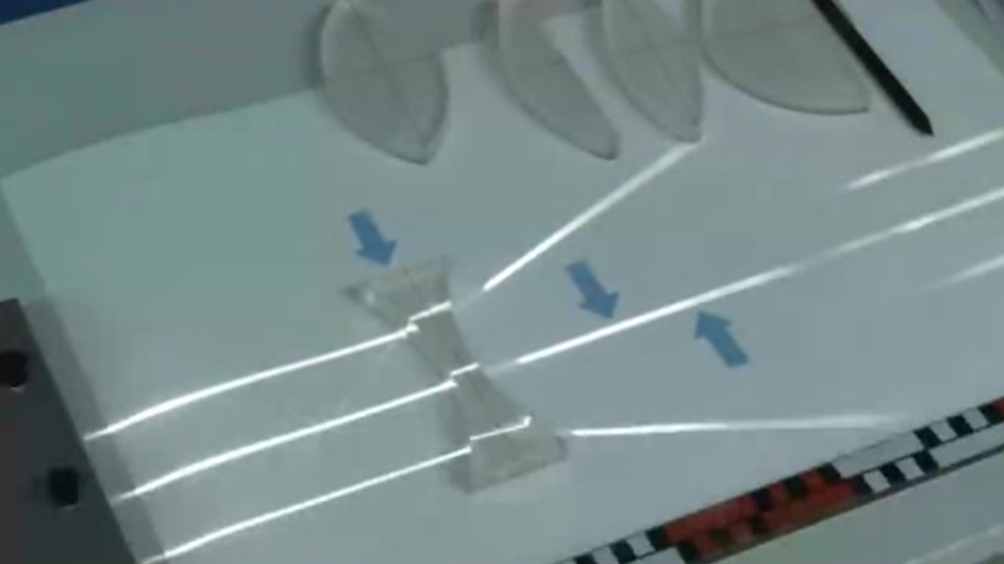
The above derived equations for a single spherical surface yield a linear relation between the input variables \(y_1\) and \(\theta_1\) and the output variables \(y_2\) and \(\theta_2\). The linear relation yields a great opportunity to express optical elements in terms of linear transformations (matrices). This is the basis of matrix optics. The matrix representation of a lens is given by

\[\begin{pmatrix} y_2 \\ \theta_2 \end{pmatrix} = \begin{pmatrix} 1 & 0 \\ -\frac{1}{f} & 1 \end{pmatrix} \begin{pmatrix} y_1 \\ \theta_1 \end{pmatrix}\]

where the matrix is called the ABCD matrix of the lens. Due to the linearization of Snells law w can write down more generally

\[\begin{pmatrix} y_2 \\ \theta_2 \end{pmatrix} = \begin{pmatrix} A & B \\ C & D \end{pmatrix} \begin{pmatrix} y_1 \\ \theta_1 \end{pmatrix}\]

and one can obtain a Matrix for all types of optical elements such as free space of dustance \(d\).

\[\begin{bmatrix} A & B\\ C & D \end{bmatrix} = \begin{bmatrix} 1 & d\\ 0 & 1 \end{bmatrix} \]

The physical meaning of the ABCD matrix elements can be understood as follows:

Element	Physical Meaning
A	Relates output height to input height (magnification-like effect)
B	Relates output height to input angle (how much an angled ray displaces)
C	Relates output angle to input height (optical power, focusing/defocusing)
D	Relates output angle to input angle (angular magnification)

Here are some useful matrices for optical elements:

\[ \mathbf{M}=\left[\begin{array}{ll} 1 & d \\ 0 & 1 \end{array}\right] \tag{Free space} \]

\[ \mathbf{M}=\left[\begin{array}{cc} 1 & 0 \\ 0 & \frac{n_1}{n_2} \end{array}\right] \tag{Planar interface} \]

\[ \mathbf{M}=\left[\begin{array}{cc} 1 & 0 \\ -\frac{\left(n_2-n_1\right)}{n_2 R} & \frac{n_1}{n_2} \end{array}\right] \tag{Spherical Boundary} \]

\[ \mathbf{M}=\left[\begin{array}{cc} 1 & 0 \\ -\frac{1}{f} & 1 \end{array}\right] \tag{Tin Lens} \]

If we have now a system of optical elements, we can multiply the matrices of the individual elements to obtain the matrix of the whole system.

\[ \rightarrow \mathrm{M}_1 \rightarrow \mathrm{M}_2 \rightarrow \mathrm{M}_N \rightarrow \mathrm{M}=\mathbf{M}_N \ldots \mathrm{M}_2 \mathbf{M}_1 \text {. } \]

This is a very powerful tool to analyze optical systems.

Example: Two-Lens System

Consider a system consisting of two thin lenses separated by a distance \(d\). The first lens has focal length \(f_1 = 100\) mm and the second lens has focal length \(f_2 = 150\) mm, separated by \(d = 200\) mm. We want to find the overall system matrix and determine where a parallel ray at height \(y_1 = 10\) mm crosses the optical axis.

The system consists of three components: 1. First lens with matrix \(\mathbf{M}_1\) 2. Free space propagation of distance \(d\) with matrix \(\mathbf{M}_{\text{free}}\) 3. Second lens with matrix \(\mathbf{M}_2\)

The individual matrices are:

\[ \mathbf{M}_1 = \begin{bmatrix} 1 & 0 \\ -\frac{1}{f_1} & 1 \end{bmatrix}, \quad \mathbf{M}_{\text{free}} = \begin{bmatrix} 1 & d \\ 0 & 1 \end{bmatrix}, \quad \mathbf{M}_2 = \begin{bmatrix} 1 & 0 \\ -\frac{1}{f_2} & 1 \end{bmatrix} \]

The total system matrix is:

\[ \mathbf{M}_{\text{total}} = \mathbf{M}_2 \cdot \mathbf{M}_{\text{free}} \cdot \mathbf{M}_1 \]

Performing the matrix multiplication:

\[ \mathbf{M}_{\text{total}} = \begin{bmatrix} 1 & 0 \\ -\frac{1}{f_2} & 1 \end{bmatrix} \begin{bmatrix} 1 & d \\ 0 & 1 \end{bmatrix} \begin{bmatrix} 1 & 0 \\ -\frac{1}{f_1} & 1 \end{bmatrix} \]

\[ = \begin{bmatrix} 1 & 0 \\ -\frac{1}{f_2} & 1 \end{bmatrix} \begin{bmatrix} 1 - \frac{d}{f_1} & d \\ -\frac{1}{f_1} & 1 \end{bmatrix} \]

\[ = \begin{bmatrix} 1 - \frac{d}{f_1} & d \\ -\frac{1}{f_2} - \frac{1}{f_1} + \frac{d}{f_1 f_2} & 1 - \frac{d}{f_2} \end{bmatrix} \]

For our specific values (\(f_1 = 100\) mm, \(f_2 = 150\) mm, \(d = 200\) mm):

\[ \mathbf{M}_{\text{total}} = \begin{bmatrix} -1 & 200 \\ -0.00333 & -0.333 \end{bmatrix} \]

For a parallel ray at height \(y_1 = 10\) mm (i.e., \(\theta_1 = 0\)):

\[ \begin{pmatrix} y_2 \\ \theta_2 \end{pmatrix} = \begin{bmatrix} -1 & 200 \\ -0.00333 & -0.333 \end{bmatrix} \begin{pmatrix} 10 \\ 0 \end{pmatrix} = \begin{pmatrix} -10 \\ -0.0333 \end{pmatrix} \]

The ray exits at height \(y_2 = -10\) mm with angle \(\theta_2 = -0.0333\) rad. The ray crosses the optical axis at a distance:

\[ b = -\frac{y_2}{\theta_2} = -\frac{-10}{-0.0333} = -300 \text{ mm} \]

This means the focal point is 300 mm before the second lens (a virtual focus). This example demonstrates how matrix optics simplifies the analysis of complex multi-element optical systems.

Thick Lens Focal Length

We would like to model the imaging properties of a thick lens using the matrix method. The lens is divided into three components:

A spherical surface at the front of the lens with radius \(R_1\)
A region of free space propagation through the lens material of thickness \(d\)
Another spherical surface at the back of the lens with radius \(R_2\)

The matrices for these components are:

\[ M_1 = \begin{bmatrix} 1 & 0 \\ -1/f_1 & 1/n \end{bmatrix}, \quad M_2 = \begin{bmatrix} 1 & d \\ 0 & 1 \end{bmatrix}, \quad M_3 = \begin{bmatrix} 1 & 0 \\ -1/f_2 & n \end{bmatrix} \]

Where - \(f_1\) and \(f_2\) are the focal lengths of the front and back surfaces, which are determined by the radii of curvature \(R_1\) and \(R_2\) of the surfaces - \(d\) is the thickness of the lens, measured along the optical axis

Derivation

For a lens with refractive index \(n\) in air, the focal lengths of the surfaces are:

\[\frac{1}{f_1} = \frac{1-n}{nR_1}, \quad \frac{1}{f_2} = \frac{n-1}{R_2}\]

Where \(R_1\) and \(R_2\) are the radii of curvature of the front and back surfaces.

The total system matrix is then

\[M_{total} = M_3 \cdot M_2 \cdot M_1\]

After multiplication the total matrix is

\[ M=\begin{bmatrix} 1 - \frac{d \left(1 - n\right)}{R_{1}} & d\\ - \frac{n-1}{R_{2} } - \frac{\left(1 - n\right) \left(n - \frac{d n \left( n-1\right)}{R_{2}}\right)}{R_{1} n} & \frac{\left(n - \frac{d n \left( n-1\right)}{R_{2}}\right)}{n} \end{bmatrix} \]

where the element in the lower left corner is the inverse of the focal length of the thick lens. This can be simplified to the following expression:

\[-\frac{1}{f} = -\frac{1}{f_2} - \frac{n}{f_1} -\frac{d n}{f_1f_2}\]

Substituting the expressions for \(1/f_1\) and \(1/f_2\):

\[\frac{1}{f} = \frac{n-1}{R_1} - \frac{n-1}{R_2} + \frac{d(n-1)^2}{nR_1R_2}\]

Factoring out \((n-1)\) gives the final expression for the focal length of a thick lens:

\[\frac{1}{f} = (n-1)\left[\frac{1}{R_1} - \frac{1}{R_2} + \frac{(n-1)d}{R_1R_2}\right]\]

This is the Lensmaker’s equation for a thick lens.

The construction of ray diagrams for thick lenses is similar to that for thin lenses, but the object and image distances are measured from the principal planes. The magnification is also calculated using the distances from the principal planes. Principal planes are where a thick lens can be treated as an equivalent thin lens. At these planes, the magnification is unity.

The derivation of the local of the principle planes will be part of the seminar.

Code

# %% Importing libraries and defining symbols
from sympy import *
from IPython.display import display, Math

n1, n2 , d, R1, R2, f1, f2, f    = symbols('n1 n2 d R1 R2 f1 f2 f')
init_session(quiet=True)
init_printing()

# %% Definition of matrices
#
f1=1/((n2-n1)/R1/n2) ## First spherical refracting surface
f2=1/((n1-n2)/R2/n1) ## Second spherical refracting surface

M1=Matrix([[1,0],[-1/f1,n1/n2]]) # first refracting surface
M2=Matrix([[1,n2*d],[0,1]]) # free space
M3=Matrix([[1,0],[-1/f2,n2/n1]]) # second refracting surface

# %% Thin lens calculation
M_thin=M3*M1  # first and second refracting surfaces
#display(Math('1/f ='+ latex(factor(collect(expand(simplify(-M_thin)[1,0]),[1/R1,1/R2],factor)))))

# The result of the matrix multiplication for a thick lens with SymPy
# %% Thick lens calculation
M_thick=M3*M2*M1

display(Math('1/f ='+ latex(collect(expand(simplify(-M_thick)[1,0]),[1/R1,1/R2,1/(R1*R2)],factor))))

\(\displaystyle 1/f =\frac{n_{1} - n_{2}}{R_{2} n_{1}} - \frac{n_{1} - n_{2}}{R_{1} n_{1}} + \frac{d \left(n_{1} - n_{2}\right)^{2}}{R_{1} R_{2} n_{1}}\)

Imaging Equation for Thick Lens

The sum of the inverse object and image distances to the principal planes (\(H_1,H_2\)) equals the inverse focal length of the thick lens:

\[\frac{1}{a}+\frac{1}{b}\approx\frac{1}{f}, \quad \text{where} \quad \frac{1}{f}=n-1\left (\frac{1}{R_1}-\frac{1}{R_2}+\frac{(n-1)d}{n R_1 R_2}\right )\]

in the paraxial approximation. The construction of the image on a thick lens is done with the help of two principle planes. The object distance \(a\) and the image distance \(b\) are measured from these principle planes. The location of the two principle planes are found to be

\[h_{1}=-\frac{(n-1)f d}{n R_2}\]

\[h_{2}=-\frac{(n-1)f d}{n R_1}\]

As compared to the construction of an image on a thin lens, we now have to consider some pecularities for the thick lens. An incident parallel ray, which turns into a focal ray is now refracted at the second principle plane. The reverse must, therefore, be true for an incident focal ray. This ray is refracted on the first principle plane. The central ray is deflected on both principle planes. It is incident under a certain angle at the first principle plane and outgoing with the same principle angle to the second principle plane. The sketch below summarizes these issues for a thick lens.

Figure 7: Thick lens image construction.

Lens types

Depending on the radii of curvature and their sign, one can construct different types of lenses that are used in many applications. Modern microscopy lenses, for example, can contain up to 20 different lenses, each with carefully designed curvatures and materials to correct for various optical aberrations and achieve high-quality imaging.