So far in our study of interference, we have focused primarily on the interaction of two waves—a useful simplification that captures the essential physics of interference phenomena. However, this two-wave picture is idealized. In most practical optical systems, we encounter situations where many partial waves interfere simultaneously. Consider a diffraction grating with thousands of parallel slits, each emitting a wavelet that contributes to the observed pattern. Or think about light bouncing back and forth between two highly reflective mirrors in a laser cavity, creating hundreds of interfering reflections. These multi-wave interference scenarios produce dramatically different and often more useful patterns than simple two-wave interference.
Understanding multiple wave interference is crucial for explaining and designing many important optical devices. Diffraction gratings, which we use for spectroscopy and wavelength measurement, rely on the interference of light from thousands of periodic sources. Fabry-Perot interferometers, used for ultra-precise wavelength measurements and laser frequency stabilization, exploit multiple reflections between parallel mirrors. Even the laser itself—perhaps the most important optical invention of the 20th century—operates through multiple wave interference in its optical cavity. The sharp, well-defined spectral lines produced by these devices, and their ability to resolve closely spaced wavelengths, all stem from the physics of multiple wave interference.
In this lecture, we will develop a general mathematical framework for analyzing multiple wave interference. We will distinguish between two important cases that arise in different physical situations. The first case involves multiple waves all having the same amplitude, as occurs in a diffraction grating where each slit contributes equally to the interference pattern. The second case involves waves with progressively decreasing amplitudes, as happens when light undergoes multiple reflections in a cavity where each reflection reduces the wave amplitude. As we’ll see, these two scenarios lead to distinctly different interference patterns with different practical applications.
Multiple Wave Interference with Constant Amplitude
Let us first consider the simpler case where multiple waves all have the same amplitude but differ in their phase. This situation occurs, for example, in a diffraction grating where light passes through many equally sized slits, or in an array of coherent sources arranged periodically. Understanding this case will provide the foundation for analyzing more complex situations.
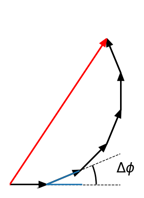
Consider \(M\) waves, each with the same amplitude but with successive phase differences. The total wave amplitude is the vector sum of all individual wave amplitudes:
\[
U=U_1+U_2+U_3+\ldots+U_M
\]
where we sum over all \(M\) partial waves. If neighboring waves (such as \(U_1\) and \(U_2\)) have a constant phase difference \(\Delta \phi\) due to, for example, a path length difference, then we can express the amplitude of the \(p\)-th wave as:
\[
U_p=\sqrt{I_0}e^{i(p-1)\Delta \phi}
\]
where \(p=1,2,\ldots,M\) is an integer index, and \(\sqrt{I_0}\) represents the amplitude of each individual wave. The total amplitude can then be written as a geometric series:
where we’ve introduced the notation \(h=e^{i\Delta \phi}\) to simplify the expression. The beauty of recognizing this as a geometric series is that we can immediately apply the closed-form sum formula to obtain:
To find the observed intensity, we must calculate the squared magnitude of this total amplitude. After factoring out appropriate phase terms and using Euler’s formula to convert complex exponentials to sines, we arrive at a remarkably elegant result:
Multiple Beam Interference Formula (Equal Amplitudes)
This formula describes the interference pattern from \(M\) waves of equal amplitude with constant phase difference \(\Delta \phi\) between neighbors.
Key features:
Numerator\(\sin^2(M\Delta \phi/2)\): oscillates \(M\) times faster than denominator
Denominator\(\sin^2(\Delta \phi/2)\): creates the envelope of the pattern
Maximum intensity: \(I_{\text{max}} = M^2 I_0\) when \(\Delta \phi = 2\pi m\) (where \(m\) is an integer)
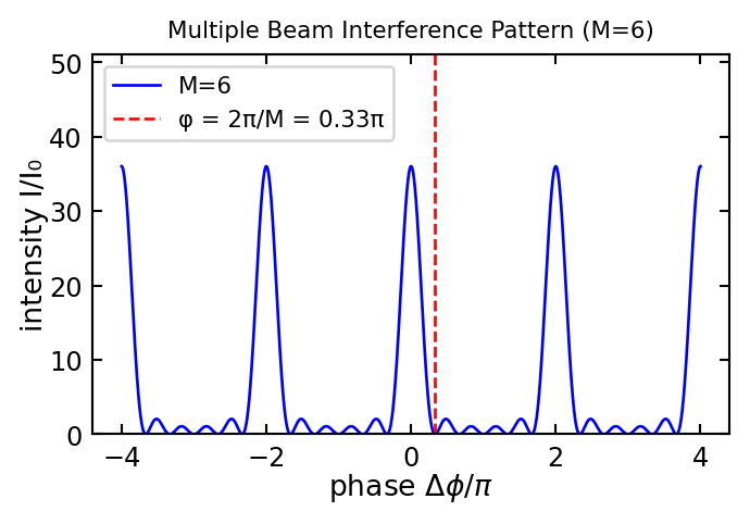
First minimum: occurs at \(\Delta \phi = 2\pi/M\)
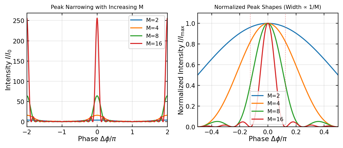
Physical interpretation: As \(M\) increases, the interference peaks become narrower and taller, while maintaining the same positions. This sharpening is crucial for high-resolution spectroscopy.
Code
# ParametersM =6# number of phasorsphi = np.pi/8# example phase difference between successive phasorsdef plot_angle(ax, pos, angle, length=0.95, acol="C0", **kwargs): vec2 = np.array([np.cos(np.deg2rad(angle)), np.sin(np.deg2rad(angle))]) xy = np.c_[[length, 0], [0, 0], vec2*length].T + np.array(pos) ax.plot(*xy.T, color=acol)return AngleAnnotation(pos, xy[0], xy[2], ax=ax, **kwargs)# Calculate phasor positionsdef calculate_phasors(phi, M):# Initialize arrays for arrow start and end points x_start = np.zeros(M) y_start = np.zeros(M) x_end = np.zeros(M) y_end = np.zeros(M)# Running sum of phasors x_sum =0 y_sum =0for i inrange(M):# Current phasor x = np.cos(i * phi) y = np.sin(i * phi)# Store start point (end of previous phasor) x_start[i] = x_sum y_start[i] = y_sum# Add current phasor x_sum += x y_sum += y# Store end point x_end[i] = x_sum y_end[i] = y_sumreturn x_start, y_start, x_end, y_endx_start, y_start, x_end, y_end = calculate_phasors(phi, M)plt.figure(figsize=get_size(6, 6))ax = plt.gca()for i inrange(M): plt.arrow(x_start[i], y_start[i], x_end[i]-x_start[i], y_end[i]-y_start[i], head_width=0.15, head_length=0.2, fc='k', ec='k', length_includes_head=True, label=f'E{i+1}'if i ==0else"")plt.arrow(0, 0, x_end[-1], y_end[-1], head_width=0.15, head_length=0.2, fc='r', ec='r', length_includes_head=True, label='Resultant')ax.set_aspect('equal')xx = np.linspace(-1, 3, 100)ax.plot(xx,(xx-1)*np.tan(phi),'k--',lw=0.5)ax.plot([1,3],[0,0],'k--',lw=0.5)kw =dict(size=195, unit="points", text=r"$\Delta \phi$")plot_angle(ax, (1.0, 0), phi*180/np.pi, textposition="inside", **kw)plt.axis('off')max_range =max(abs(x_end[-1]), abs(y_end[-1])) *1.2plt.xlim(-0, max_range/1.5)plt.ylim(-0.1, max_range/1.)plt.show()# ParametersM =6phi = np.linspace(-4*np.pi, 4*np.pi, 10000) # increased resolutionI0 =1def multiple_beam_pattern(phi, M): numerator = np.sin(M * phi/2)**2 denominator = np.sin(phi/2)**2 I = np.where(denominator !=0, numerator/denominator, M**2)return II = I0 * multiple_beam_pattern(phi, M)first_min =2*np.pi/M # theoretical valuedef find_nearest(array, value): array = np.asarray(array) idx = (np.abs(array - value)).argmin()return array[idx], idxhalf_max = M**2/2phi_positive = phi[phi >=0] # only positive valuesI_positive = I[phi >=0]_, idx_half = find_nearest(I_positive, half_max)half_width = phi_positive[idx_half]# Create plotplt.figure(figsize=get_size(10, 6))plt.plot(phi/np.pi, I, 'b-', label=f'M={M}')#plt.plot(first_min/np.pi, multiple_beam_pattern(first_min, M), 'ro')#plt.annotate(f'First minimum\nφ = 2π/M = {first_min/np.pi:.2f}π',plt.axvline(x=first_min/np.pi, color='r', linestyle='--', label=f'φ = 2π/M = {first_min/np.pi:.2f}π')#plt.plot(half_width/np.pi, half_max, 'go')plt.xlabel(r'phase $\Delta \phi/\pi$')plt.ylabel('intensity I/I₀')plt.title(f'Multiple Beam Interference Pattern (M={M})')plt.ylim(0, M**2+15)plt.legend()plt.show()
Multiple wave interference of \(M=6\) waves with a phase difference of \(\phi=\pi/8\). The black arrows represent the individual waves, the red arrow the sum of all waves.
Figure 1— Multiple beam interference pattern for M=6 beams. The intensity distribution is shown as a function of the phase shift \(\phi\). The first minimum is at \(\phi=2\pi/M\). The intensity distribution is symmetric around \(\phi=0\).
This intensity formula reveals several fascinating features. The numerator \(\sin^2(M\Delta \phi/2)\) oscillates with a frequency that is \(M\) times higher than the denominator \(\sin^2(\Delta \phi/2)\). This creates a rapidly oscillating pattern that produces sharp interference peaks separated by regions of low intensity. The first minimum of the interference peak occurs at \(\Delta \phi = 2\pi/M\), which is a crucial result: it shows that the number of sources \(M\) directly determines how narrow the interference peak becomes. As we add more sources, the peaks become increasingly sharp and well-defined.
This narrowing effect has profound practical implications. In a diffraction grating with spacing \(d\) between adjacent slits, the phase difference between neighboring sources is \(\Delta \phi = 2\pi d \sin(\theta)/\lambda\), just as in the double-slit experiment. Using this relationship, we can express the angular width of the interference peak. The first minimum occurs at an angle given by:
Notice that this angular width is inversely proportional to the total width of the grating (\(Md\)), not just to the slit spacing \(d\). A grating with 10,000 slits produces peaks that are 10,000 times narrower than a double-slit with the same spacing! This is why diffraction gratings can resolve spectral lines that are extremely close in wavelength—a capability essential for spectroscopy in chemistry, astronomy, and materials science.
A mathematically subtle but physically important situation arises when both the numerator and denominator simultaneously approach zero. This occurs whenever the phase difference is an integer multiple of \(2\pi\):
\[
\Delta \phi = 2\pi m
\]
where \(m\) is an integer called the interference order, representing how many wavelengths of path difference exist between neighboring partial waves. At these special points, our formula appears to give the indeterminate form \(0/0\). However, applying L’Hôpital’s rule or using the small-angle approximation for the sine functions reveals that:
\[
I(\Delta \phi = 2\pi m) = M^2 I_0
\]
This is the maximum possible intensity, and it’s proportional to the square of the number of sources. This quadratic scaling is remarkable: doubling the number of sources quadruples the peak intensity. This explains why diffraction gratings with many lines are so much brighter and more efficient than simple double slits.
Code
# Parametersphi = np.linspace(-2*np.pi, 2*np.pi, 5000)I0 =1M_values = [2, 4, 8, 16]colors = ['#1f77b4', '#ff7f0e', '#2ca02c', '#d62728']fig, (ax1, ax2) = plt.subplots(1, 2, figsize=get_size(18, 8))# Left plot: All on same scalefor M, color inzip(M_values, colors):def multiple_beam_pattern(phi, M): numerator = np.sin(M * phi/2)**2 denominator = np.sin(phi/2)**2 I = np.where(denominator !=0, numerator/denominator, M**2)return I I = I0 * multiple_beam_pattern(phi, M) ax1.plot(phi/np.pi, I, label=f'M={M}', color=color, linewidth=1.5)ax1.set_xlabel(r'Phase $\Delta\phi/\pi$')ax1.set_ylabel(r'Intensity $I/I_0$')ax1.set_title('Peak Narrowing with Increasing M')ax1.legend()ax1.grid(True, alpha=0.3)ax1.set_xlim(-2, 2)# Right plot: Normalized to show shape (divide by M^2)for M, color inzip(M_values, colors): I = I0 * multiple_beam_pattern(phi, M) / (M**2) ax2.plot(phi/np.pi, I, label=f'M={M}', color=color, linewidth=1.5)# Mark FWHM for M=16if M ==16:# Find first minimum first_min =2*np.pi/M ax2.axvline(x=first_min/np.pi, color=color, linestyle=':', alpha=0.5, linewidth=1) ax2.axvline(x=-first_min/np.pi, color=color, linestyle=':', alpha=0.5, linewidth=1)ax2.set_xlabel(r'Phase $\Delta\phi/\pi$')ax2.set_ylabel(r'Normalized Intensity $I/I_{\rm max}$')ax2.set_title('Normalized Peak Shapes (Width ∝ 1/M)')ax2.legend()ax2.grid(True, alpha=0.3)ax2.set_xlim(-0.5, 0.5)ax2.set_ylim(0, 1.1)plt.tight_layout()plt.show()
Figure 2— Comparison of interference patterns for different numbers of sources M. As M increases, the peaks become narrower and taller while maintaining the same position. This demonstrates the fundamental principle underlying diffraction grating spectroscopy.
Application: Diffraction Gratings
The multiple beam interference formula we’ve derived provides the theoretical foundation for one of the most important optical instruments: the diffraction grating. A diffraction grating consists of many parallel slits or lines (typically thousands) with regular spacing \(d\). When illuminated by light, each slit acts as a coherent source, and the interference of light from all these sources creates sharp, bright spectral lines at specific angles determined by the wavelength through the grating equation \(\sin(\theta_m) = m\lambda/d\).
The key result from our interference analysis is that the angular width of each spectral peak is inversely proportional to the total number of illuminated grating lines \(M\). This leads to the resolving power \(R = mM\), where \(m\) is the diffraction order. More slits create sharper peaks, enabling better separation of closely spaced wavelengths—the fundamental principle of spectroscopic analysis.
Further Study: Diffraction Gratings
The detailed physics of diffraction gratings, including the combined effects of single-slit diffraction and multi-slit interference, is covered in a dedicated lecture after we study diffraction. Topics include:
Complete grating equation including diffraction envelope
Spectral resolution and resolving power
Influence of slit width and number on the diffraction pattern
Practical applications in spectroscopy and optical instruments
Real experimental observations and design considerations
The interference theory developed here provides the foundation for understanding how gratings create their characteristic sharp spectral lines.
Calculation: Interference of M Waves with Different Frequencies
Consider \(M\) waves with equal amplitudes but different frequencies, where the frequencies are equally spaced by \(\Delta\nu\) around a central frequency \(\nu_0\). The \(p\)-th wave can be written as:
This result shows that the intensity oscillates in time with a period \(T = 1/\Delta\nu\), reaching maximum intensity \(I_{\max} = M^2 I_0\) when \(\Delta\nu t = m\) (integer \(m\)). The temporal beating pattern becomes sharper as \(M\) increases—a frequency-domain analog of the spatial interference pattern from a diffraction grating. This phenomenon is exploited in frequency combs and mode-locked lasers.
Wavevector Representation: A Powerful Geometric Insight
There is an elegant geometric way to understand multiple wave interference using wavevectors that provides deep insight into the physics and connects to many other phenomena in optics and solid-state physics. Let’s rewrite the first-order (\(m=1\)) constructive interference condition in terms of wavevectors rather than wavelengths and angles.
The standard grating equation \(d\sin\theta = \lambda\) can be rewritten by dividing both sides by the wavelength:
\(k = 2\pi/\lambda\) is the magnitude of the wavevector of the light
\(K = 2\pi/d\) is the grating wavevector corresponding to the grating period \(d\)
\(\theta\) is the diffraction angle
Deriving the vector form: To understand the vector notation, consider the geometry of diffraction. The incident light has wavevector \(\vec{k}_{\text{in}}\) (horizontal in our setup), and the diffracted light has wavevector \(\vec{k}_{\text{out}}\) at angle \(\theta\) from the horizontal. Both wavevectors have the same magnitude \(k = 2\pi/\lambda\) since the wavelength doesn’t change during elastic scattering.
The change in the wavevector is \(\Delta\vec{k} = \vec{k}_{\text{out}} - \vec{k}_{\text{in}}\). Since both wavevectors have magnitude \(k\), we can decompose them:
The change in wavevector is therefore: \[\Delta\vec{k} = k(\cos\theta - 1)\hat{x} + k\sin\theta\,\hat{y}\]
The vertical component of the wavevector change is: \(\Delta k_y = k\sin\theta\). From our scalar equation, this equals \(K = 2\pi/d\).
Important note on the vector equation: You might be tempted to write the simple vector equation: \[\vec{k}_{\text{out}} = \vec{k}_{\text{in}} + \vec{K}\]
However, this is only an approximation valid for small diffraction angles! Here’s why: if we literally add \(\vec{k}_{\text{in}} = k\hat{x}\) and \(\vec{K} = K\hat{y}\), the resulting magnitude would be \(\sqrt{k^2 + K^2} \neq k\), which violates elastic scattering.
The exact condition: The diffraction must satisfy both: 1. The grating equation: \(k\sin\theta = K\) (perpendicular momentum transfer) 2. Elastic scattering: \(|\vec{k}_{\text{out}}| = |\vec{k}_{\text{in}}| = k\) (energy conservation)
This gives the exact result: \[\vec{k}_{\text{out}} = \sqrt{k^2-K^2}\,\hat{x} + K\hat{y} = k\cos\theta\,\hat{x} + k\sin\theta\,\hat{y}\]
Note the horizontal component: \(\sqrt{k^2-K^2} = k\cos\theta < k\).
When the approximation works: For small angles where \(K \ll k\) (equivalently \(\sin\theta \ll 1\)): - \(\sqrt{k^2-K^2} \approx k - K^2/(2k) \approx k\) - The horizontal component change \(k\cos\theta - k \approx -K^2/(2k)\) is negligible - Then \(\vec{k}_{\text{out}} \approx \vec{k}_{\text{in}} + \vec{K}\) becomes a good approximation
For typical gratings in visible light, diffraction angles are indeed small (a few degrees), so this approximation is often reasonable for intuitive understanding.
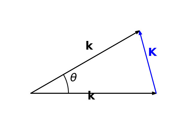
Geometric interpretation: The grating provides a momentum transfer with perpendicular component \(K\). The incident and diffracted wavevectors (both with magnitude \(k\)), together with the change in wavevector, form a vector triangle. Because elastic scattering constrains both \(|\vec{k}_{\text{in}}| = |\vec{k}_{\text{out}}| = k\), this forms an isosceles triangle. The grating equation \(k\sin\theta = K\) determines the geometry of this triangle. This is momentum conservation: the periodic grating structure transfers momentum to the light in discrete units determined by the grating period.
Universal principle: This wavevector conservation principle applies throughout wave physics: X-ray diffraction from crystals (Bragg’s law), electron diffraction, neutron scattering, phonon interactions, and even particle scattering in quantum mechanics—wherever periodic structures interact with waves.
Since the magnitude of the light’s wavevector is conserved (elastic scattering), the incident and diffracted wavevectors both have magnitude \(k\). Together with the change in wavevector \(\Delta\vec{k}\), they form an isosceles triangle, as shown in the figure below. The perpendicular component of this momentum change has magnitude \(K\). This geometric picture reveals that the grating is effectively providing a “momentum kick” perpendicular to its surface to change the light’s direction. This same wavevector conservation principle appears throughout physics: in X-ray diffraction from crystals (the Bragg condition), in electron diffraction, in the scattering of light by acoustic waves, and even in nonlinear optics where photons combine or split.
Wavevector summation for the diffraction grating. The wavevector of the incident light \(k\) and the wavevector of the light traveling along the direction of the first interference peak \(K\) form an equilateral triangle.
This means that the diffraction grating is providing a momentum transfer with perpendicular component \(K\) to alter the direction of the incident light. The constraint that both incident and diffracted light have the same wavevector magnitude \(k\) (elastic scattering) determines the exact geometry. This wavevector conservation principle reappears throughout physics, for example in X-ray diffraction from crystals (where it leads to Bragg’s law).
Multiple Wave Interference with Decreasing Amplitude
We now turn our attention to a physically important variation of multiple wave interference: the case where successive waves have progressively decreasing amplitudes. This scenario arises naturally whenever light undergoes multiple reflections in an optical cavity, such as in a Fabry-Perot interferometer or the mirrors of a laser cavity. Each time light reflects from a partially reflective surface, only a fraction of the amplitude is reflected—the rest is transmitted through the surface and lost from the interference pattern within the cavity.
Consider a sequence of waves where the first wave has amplitude \(U_1 = \sqrt{I_0}\), but each subsequent wave has its amplitude reduced by a constant factor. We express the second wave as:
\[
U_2=h U_1
\]
where \(h = re^{i\Delta\phi}\) with \(|h| = r < 1\). Here \(r\) represents the reflection coefficient, a dimensionless number less than one that describes what fraction of the wave amplitude survives each reflection. The phase factor \(e^{i\Delta\phi}\) accounts for the additional optical path traveled between successive reflections. When we calculate the intensity of this second wave, we find:
\[
I_2=|U_2|^2=|h U_1|^2=r^2 I_1
\]
This reveals an important distinction: while the amplitude is multiplied by \(r\) at each reflection, the intensity is multiplied by \(r^2\). The phase factor \(e^{i\Delta\phi}\) vanishes when we take the squared magnitude to find intensity, as \(|e^{i\Delta\phi}|^2 = 1\). This means the phase affects where the waves interfere, but the factor \(r\) determines how quickly the wave amplitudes decay with successive reflections.
Reflectance, Transmittance, and Energy Conservation
The amplitude reflection coefficient \(r \le 1\) determines what fraction of the wave amplitude is reflected at a boundary. The corresponding reflectance\(R = |r|^2 \le 1\) gives the fraction of intensity (energy per unit area per unit time) that is reflected.
The transmittance\(T\) is the fraction of intensity transmitted through the boundary. In the absence of absorption, energy conservation requires:
\[
R+T=1
\]
Example: A typical uncoated glass surface has \(R \approx 0.04\) (4% reflectance) and \(T \approx 0.96\) (96% transmittance). High-quality mirror coatings can achieve \(R > 0.999\) (99.9% reflectance).
Forward reference: The Airy function and concepts of finesse developed here form the theoretical foundation for understanding Fabry-Perot interferometers, which are covered in detail in a separate dedicated lecture on Fabry-Perot interferometry.
Following this pattern, the third wave has amplitude \(U_3 = hU_2 = h^2U_1\), the fourth has \(U_4 = h^3U_1\), and so on. If we sum over many such reflections (potentially infinite in number), the total amplitude becomes:
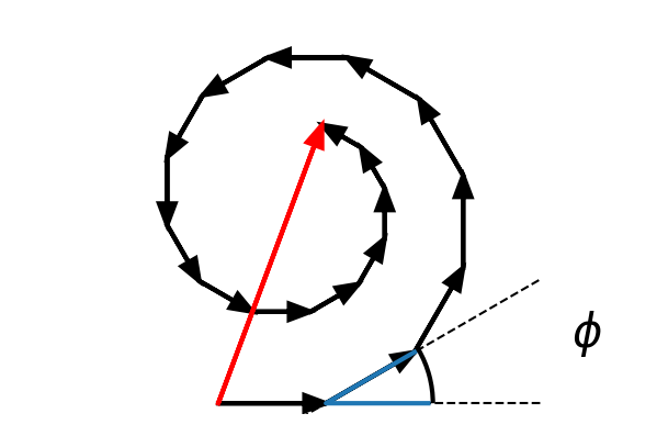
M =18# number of phasorsphi = np.pi/6# example phase difference between successive phasorsr =0.95# reduction factor for each subsequent phasordef plot_angle(ax, pos, angle, length=0.95, acol="C0", **kwargs): vec2 = np.array([np.cos(np.deg2rad(angle)), np.sin(np.deg2rad(angle))]) xy = np.c_[[length, 0], [0, 0], vec2*length].T + np.array(pos) ax.plot(*xy.T, color=acol)return AngleAnnotation(pos, xy[0], xy[2], ax=ax, **kwargs)def calculate_phasors(phi, M, r): x_start = np.zeros(M) y_start = np.zeros(M) x_end = np.zeros(M) y_end = np.zeros(M) x_sum =0 y_sum =0for i inrange(M): amplitude = r**i # exponential decrease x = amplitude * np.cos(i * phi) y = amplitude * np.sin(i * phi) x_start[i] = x_sum y_start[i] = y_sum x_sum += x y_sum += y x_end[i] = x_sum y_end[i] = y_sumreturn x_start, y_start, x_end, y_endx_start, y_start, x_end, y_end = calculate_phasors(phi, M, r)plt.figure(figsize=get_size(6, 6),dpi=150)ax = plt.gca()for i inrange(M): plt.arrow(x_start[i], y_start[i], x_end[i]-x_start[i], y_end[i]-y_start[i], head_width=0.15, head_length=0.2, fc='k', ec='k', length_includes_head=True, label=f'E{i+1}'if i ==0else"")plt.arrow(0, 0, x_end[-1], y_end[-1], head_width=0.15, head_length=0.2, fc='r', ec='r', length_includes_head=True, label='Resultant')ax.set_aspect('equal')xx = np.linspace(-1, 3, 100)ax.plot(xx,(xx-1)*np.tan(phi),'k--',lw=0.5)ax.plot([1,3],[0,0],'k--',lw=0.5)kw =dict(size=195, unit="points", text=r"$\phi$")plot_angle(ax, (1.0, 0), phi*180/np.pi, textposition="inside", **kw)plt.axis('off')max_range =max(abs(x_end[-1]), abs(y_end[-1])) *1.2plt.xlim(-max_range/1.8, max_range/0.8)plt.ylim(-0.1, max_range/0.9)plt.show()import numpy as npimport matplotlib.pyplot as plt# Create phase array from -2π to 2πphi = np.linspace(-2*np.pi, 2*np.pi, 1000)def calculate_intensity(phi, F):return1/(1+4*(F/np.pi)**2* np.sin(phi/2)**2)plt.figure(figsize=get_size(10, 6))finesse_values = [1, 4, 20]styles = ['-', '--', ':']for F, style inzip(finesse_values, styles): I = calculate_intensity(phi, F) plt.plot(phi/np.pi, I, style, label=f'$\\mathcal{{F}}={F}$')plt.xlabel('Phase $\\phi/\\pi$')plt.ylabel('$I/I_{\\mathrm{max}}$')plt.grid(True, alpha=0.3)plt.legend()plt.ylim(0, 1.1)plt.show()
Phase construction of a multiwave intereference with M waves with decreasing amplitude due to a reflection coefficient \(r=0.95\).
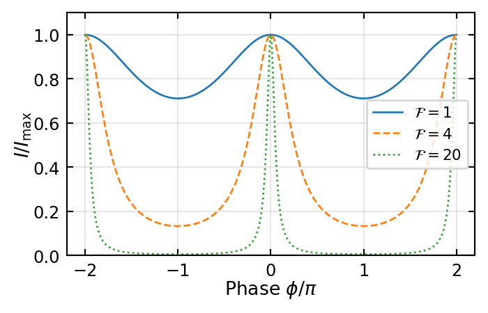
Multiple wave interference with decreasing amplitude. The graph shows the intensity distribution over the phase angle \(\phi\) for different values of the Finesse \(\mathcal{F}\).
This is again a geometric series, which we can sum using the standard formula (taking the limit as \(M \to \infty\) since reflections continue indefinitely):
This fundamental result is known as the Airy function or Airy formula, named after the British astronomer George Biddell Airy who first derived it in 1833 while studying the properties of spectroscopic instruments.
The finesse \(\mathcal{F}\) is perhaps the most important parameter characterizing a Fabry-Perot cavity or any resonant optical system. It quantifies how “sharp” the resonance peaks are compared to their spacing. A cavity with highly reflective mirrors (say \(r = 0.99\), giving \(R = 98\%\) reflectance) has a finesse of about \(\mathcal{F} \approx 310\), producing extremely narrow transmission peaks. This makes such cavities exquisitely sensitive to small changes in wavelength or cavity length.
The intensity distribution described by the Airy function has a profoundly different character from the equal-amplitude case. As we increase the finesse, the intensity maxima—which occur at multiples of \(2\pi\) in phase—become dramatically narrower and more isolated. Between the maxima, the intensity drops to nearly zero, creating regions of almost complete destructive interference. This sharp wavelength selectivity makes Fabry-Perot interferometers indispensable for applications requiring ultra-high spectral resolution, such as measuring the frequency stability of lasers, detecting tiny Doppler shifts in astrophysics, and studying the fine structure of atomic emission lines.
Connection to Fabry-Perot Interferometry
The Airy function we’ve derived is the fundamental intensity distribution for any optical system involving multiple reflections with decreasing amplitude. The most important practical realization of this physics is the Fabry-Perot interferometer, which consists of two parallel, partially reflective mirrors separated by a distance \(L\). When light enters this cavity, it bounces back and forth many times, with each reflection reducing the amplitude by the factor \(r\), creating exactly the scenario we’ve analyzed.
The Fabry-Perot interferometer exhibits transmission peaks whenever the round-trip phase satisfies \(\Delta\phi = 4\pi L/\lambda = 2\pi m\), corresponding to cavity lengths that are integer multiples of half-wavelengths. The sharpness of these peaks—characterized by the finesse—makes Fabry-Perot devices essential for applications requiring ultra-high spectral resolution, such as laser frequency stabilization, precision spectroscopy, and optical communications.
Further Study: Fabry-Perot Interferometers
The detailed physics, applications, and experimental techniques of Fabry-Perot interferometry are covered in a dedicated lecture. Topics include:
Free spectral range and spectral resolution
Ring pattern formation and interpretation
Applications in spectroscopy, laser technology, and optical communications
Modern implementations in photonics and quantum optics
The Airy function and finesse concepts developed here provide the theoretical foundation for understanding these practical devices.
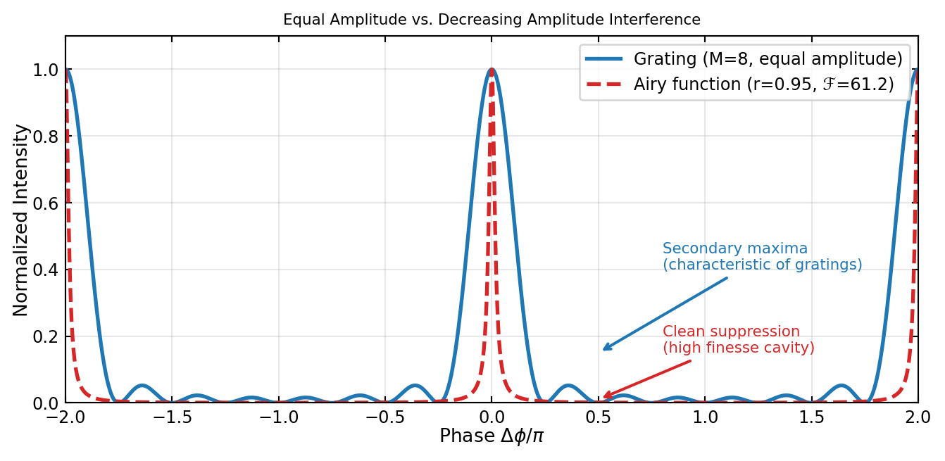
Figure 3— Comparison between equal-amplitude interference (diffraction grating, blue) and decreasing-amplitude interference (Airy function with high finesse, red). The grating shows secondary maxima between main peaks, while the Airy function shows clean suppression between resonances - a key distinction exploited in Fabry-Perot interferometers.
Conclusion: From Fundamental Physics to Precision Technology
The transition from two-wave to multiple-wave interference represents more than just mathematical generalization—it reveals a profound principle that underpins much of modern photonics. When many coherent sources interfere, whether they have equal amplitudes (as in diffraction gratings) or decreasing amplitudes (as in Fabry-Perot cavities and laser resonators), the resulting patterns exhibit dramatically sharper features than simple two-wave interference. This sharpening effect, characterized mathematically by the \(M^2\) intensity scaling in gratings and the finesse parameter in the Airy function, provides the foundation for optical instruments of extraordinary precision and capability.
Diffraction gratings, exploiting the equal-amplitude interference of thousands of sources, have become indispensable tools for separating and analyzing light. As we’ll explore in detail in the dedicated lecture on diffraction gratings, these devices combine the interference principles developed here with single-slit diffraction effects to create powerful spectroscopic instruments used throughout science and technology—from astronomical spectroscopy revealing the composition of distant stars to compact spectrometers in chemistry labs and wavelength-division multiplexing in optical communications.
The Airy function, describing interference with decreasing amplitudes, governs systems where waves undergo multiple reflections in optical cavities. As we’ll see in the dedicated lecture on Fabry-Perot interferometry, this physics enables wavelength measurements accurate to parts per billion, frequency stabilization of lasers to better than one part in \(10^{15}\), and spectroscopic resolution sufficient to observe individual spectral components separated by only megahertz. The remarkably narrow transmission peaks of high-finesse cavities make Fabry-Perot devices essential for applications ranging from laser technology and precision spectroscopy to optical communications and quantum optics.
The mathematical frameworks we’ve developed—the multi-beam formula for equal amplitudes and the Airy function for decreasing amplitudes—appear throughout physics wherever periodic structures interact with waves. The same wavevector addition that describes grating diffraction also governs X-ray scattering from crystal lattices (Bragg diffraction), the electronic band structure of semiconductors, and even the propagation of light in photonic crystals that act as “semiconductors for photons.” Understanding multiple wave interference thus provides not just isolated techniques for optical measurements, but a universal language for describing how waves interact with periodic structures across all scales and all branches of physics.