Polarization of Light
Introduction: The Nature of Polarization
Light is a transverse electromagnetic wave: the electric field oscillates perpendicular to the propagation direction. Since nearly all interactions of light with matter, from refraction and absorption to detection, are governed by the electric field, the way this field oscillates in space and time is a central property of light. We call it the polarization state.
Polarization is fundamentally important in photonics:
- Optical communication: Polarization-division multiplexing (PDM) increases bandwidth
- Display technology: Liquid crystal displays (LCDs) rely on polarization control
- Stress analysis: Photoelasticity uses polarized light to visualize strain
- Quantum optics: Single photons carry quantum information in polarization
- Remote sensing: Depolarization indicates atmospheric properties
This lecture develops the mathematical formalism to describe and manipulate light polarization, in three stages: the real field description, the Jones calculus for fully polarized light, and the Stokes description that also covers partially polarized light.
Electromagnetic Waves and Polarization
The Wave Equation from Maxwell’s Equations
Starting from Maxwell’s equations in vacuum:
\[\nabla \times \mathbf{E} = -\frac{\partial \mathbf{B}}{\partial t}\] \[\nabla \times \mathbf{B} = \mu_0 \epsilon_0 \frac{\partial \mathbf{E}}{\partial t}\]
Taking the curl of the first equation, using the vector identity \(\nabla \times (\nabla \times \mathbf{E}) = \nabla(\nabla \cdot \mathbf{E}) - \nabla^2 \mathbf{E}\) together with \(\nabla \cdot \mathbf{E} = 0\) in vacuum, and inserting the second equation yields:
\[\nabla^2 \mathbf{E} = \mu_0 \epsilon_0 \frac{\partial^2 \mathbf{E}}{\partial t^2} \tag{1}\]
This is the wave equation, with wave speed \(c = 1/\sqrt{\mu_0 \epsilon_0}\).
Plane Wave Solutions
For a plane wave propagating in the \(+z\) direction:
\[\mathbf{E}(z,t) = \mathbf{E}_0 \cos(kz - \omega t + \phi)\]
where \(k = 2\pi/\lambda\) is the wavenumber and \(\omega = 2\pi f\) is the angular frequency. Gauss’s law \(\nabla \cdot \mathbf{E} = 0\) requires \(\mathbf{k} \cdot \mathbf{E}_0 = 0\): the field has no component along the propagation direction. A plane wave therefore has exactly two independent transverse components:
\[E_x(z,t) = E_{0x} \cos(kz - \omega t + \phi_x)\] \[E_y(z,t) = E_{0y} \cos(kz - \omega t + \phi_y) \tag{2}\]
At a fixed position (\(z = 0\)):
\[E_x(t) = E_{0x} \cos(\omega t - \phi_x)\] \[E_y(t) = E_{0y} \cos(\omega t - \phi_y)\]
Both components oscillate at the same frequency, so the polarization state is completely characterized by just three numbers: the two amplitudes \(E_{0x}\), \(E_{0y}\) and the relative phase
\[\delta = \phi_y - \phi_x .\]
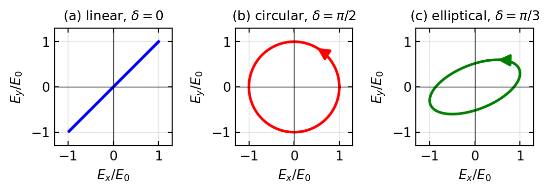
Depending on these values, the tip of the electric field vector traces a line, a circle, or an ellipse in the transverse plane.
Polarization States
Linear Polarization
When \(\delta = 0\) or \(\delta = \pi\), the two components oscillate in step (or exactly in counter-step), and
\[E_y = \pm\frac{E_{0y}}{E_{0x}} E_x ,\]
with the \(+\) sign for \(\delta = 0\) and the \(-\) sign for \(\delta = \pi\). The electric field vector oscillates along a straight line in the \(xy\) plane, inclined at the angle \(\theta = \arctan(\pm E_{0y}/E_{0x})\) to the \(x\) axis.
Circular Polarization
When \(E_{0x} = E_{0y} = E_0\) and \(\delta = +\pi/2\):
\[E_x(t) = E_0 \cos(\omega t)\] \[E_y(t) = E_0 \sin(\omega t)\]
The electric field vector rotates with constant magnitude \(E_0\): at \(t = 0\) it points along \(+x\), a quarter period later along \(+y\). An observer facing the oncoming beam (looking back toward the source) sees the field rotate clockwise; this is called right circular polarization (RCP) in the convention of Hecht and Born & Wolf, which we adopt throughout. With \(\delta = -\pi/2\) the rotation reverses and the light is left circular (LCP). Be warned that the opposite naming convention also appears in the literature, so always check which one a book or data sheet uses.
Elliptical Polarization
For arbitrary amplitudes and phases, eliminating \(t\) from the two component equations gives
\[\left(\frac{E_x}{E_{0x}}\right)^2 + \left(\frac{E_y}{E_{0y}}\right)^2 - 2\,\frac{E_x E_y}{E_{0x} E_{0y}}\cos\delta = \sin^2\delta ,\]
the equation of an ellipse. The tip of the field vector traces this ellipse once per optical period. Linear and circular polarization are simply the degenerate special cases (\(\sin\delta = 0\) collapses the ellipse to a line; equal amplitudes with \(\delta = \pm\pi/2\) make it a circle). Figure 1 shows the three cases.
The Jones Vector Formalism
Carrying the two amplitudes and the phase around in trigonometric form quickly becomes clumsy. Since both components oscillate at the same frequency \(\omega\), we can drop the common time dependence and collect amplitude and phase of each component into a complex number. The Jones vector represents a fully polarized plane wave:
\[\mathbf{J} = \begin{pmatrix} E_x \\ E_y \end{pmatrix} = \begin{pmatrix} E_{0x} e^{-i\phi_x} \\ E_{0y} e^{-i\phi_y} \end{pmatrix} \tag{3}\]
The real field is recovered as \(\mathbf{E}(t) = \mathrm{Re}[\mathbf{J}\, e^{i\omega t}]\). A global phase factor multiplying \(\mathbf{J}\) has no physical significance; only the amplitude ratio and the relative phase \(\delta\) matter. Jones vectors are usually normalized so that \(|\mathbf{J}|^2 = 1\).
Common Jones Vectors
Horizontal: \(\mathbf{J}_H = \begin{pmatrix} 1 \\ 0 \end{pmatrix}\), Vertical: \(\mathbf{J}_V = \begin{pmatrix} 0 \\ 1 \end{pmatrix}\), Linear at angle \(\theta\): \(\mathbf{J}_\theta = \begin{pmatrix} \cos\theta \\ \sin\theta \end{pmatrix}\)
Right circular: \(\mathbf{J}_{RCP} = \frac{1}{\sqrt{2}} \begin{pmatrix} 1 \\ -i \end{pmatrix}\), Left circular: \(\mathbf{J}_{LCP} = \frac{1}{\sqrt{2}} \begin{pmatrix} 1 \\ i \end{pmatrix}\)
The circular vectors follow directly from the previous section: RCP has \(\delta = +\pi/2\), so \(E_{0y}e^{-i\phi_y} = e^{-i\pi/2} = -i\) relative to the \(x\) component. Note that \(\mathbf{J}_H \cdot \mathbf{J}_V^* = 0\) and \(\mathbf{J}_{RCP} \cdot \mathbf{J}_{LCP}^* = 0\): both pairs form orthogonal bases, and any polarization state can be decomposed in either basis.
Intensity: \(I \propto |\mathbf{J}|^2 = |E_x|^2 + |E_y|^2\)
Jones Matrices and Optical Elements
Every linear, non-depolarizing optical element transforms the Jones vector by a \(2\times 2\) matrix, \(\mathbf{J}_\text{out} = M\, \mathbf{J}_\text{in}\). A sequence of elements multiplies from the right to the left, in the order the light encounters them:
\[\mathbf{J}_\text{out} = M_N \cdots M_2\, M_1\, \mathbf{J}_\text{in}\]
Polarizers
A polarizer projects the field onto its transmission axis:
Horizontal: \(M_H = \begin{pmatrix} 1 & 0 \\ 0 & 0 \end{pmatrix}\), Vertical: \(M_V = \begin{pmatrix} 0 & 0 \\ 0 & 1 \end{pmatrix}\)
At angle \(\theta\): \(M(\theta) = \begin{pmatrix} \cos^2\theta & \cos\theta\sin\theta \\ \cos\theta\sin\theta & \sin^2\theta \end{pmatrix}\) {#eq-jones-polarizer}
The matrix \(M(\theta) = \mathbf{J}_\theta \mathbf{J}_\theta^\dagger\) is exactly the projection operator onto the direction \(\theta\).
Retardance Plates
A retarder (wave plate) is made of a birefringent material: light polarized along the fast axis travels with a lower refractive index than light along the perpendicular slow axis. After the plate, the slow component lags by the retardance phase \(\Gamma\). With the fast axis along \(x\), the Jones matrix is, up to a global phase,
\[M_\text{ret}(\Gamma) = \begin{pmatrix} 1 & 0 \\ 0 & e^{-i\Gamma} \end{pmatrix}\]
The two most important special cases are the quarter-wave plate (QWP, \(\Gamma = \pi/2\)) and the half-wave plate (HWP, \(\Gamma = \pi\)):
\[M_{QWP} = \begin{pmatrix} 1 & 0 \\ 0 & -i \end{pmatrix}, \qquad M_{HWP} = \begin{pmatrix} 1 & 0 \\ 0 & -1 \end{pmatrix}\]
For an element whose fast axis is rotated by an angle \(\theta\), transform into the element frame and back with the rotation matrix \(R(\theta) = \begin{pmatrix} \cos\theta & -\sin\theta \\ \sin\theta & \cos\theta \end{pmatrix}\):
\[M(\theta) = R(\theta)\, M\, R(-\theta)\]
For the half-wave plate at angle \(\alpha\) this evaluates to the simple real matrix
\[M_{HWP}(\alpha) = \begin{pmatrix} \cos 2\alpha & \sin 2\alpha \\ \sin 2\alpha & -\cos 2\alpha \end{pmatrix},\]
which maps linear polarization at angle \(\theta\) to linear polarization at angle \(2\alpha - \theta\): the HWP mirrors the polarization direction about its fast axis, and therefore rotates linear polarization by twice the angle between the input polarization and the fast axis.
Worked Example: Producing Circular Light
The standard laboratory recipe for circular polarization is linear input at \(45°\) to the fast axis of a quarter-wave plate. The two equal components then acquire a \(\pi/2\) relative phase, which is precisely the definition of circular light:
Code
import numpy as np

# Jones matrices (fast axis horizontal)
M_qwp = np.array([[1, 0], [0, -1j]], dtype=complex)   # quarter-wave plate

# Input: linear polarization at 45 degrees
J_in = np.array([1, 1], dtype=complex) / np.sqrt(2)
print("Input intensity: ", np.sum(np.abs(J_in)**2).real)

# Output after the QWP
J_out = M_qwp @ J_in
print("Output Jones vector:", J_out)
print("Output intensity:", np.sum(np.abs(J_out)**2).real)
Input intensity: 0.9999999999999998
Output Jones vector: [0.70710678+0.j 0. -0.70710678j]
Output intensity: 0.9999999999999998The output \((1, -i)/\sqrt{2}\) is the right circular state \(\mathbf{J}_{RCP}\). The intensity is unchanged because a retarder only shifts phases; it absorbs no light. Sending the same input through a half-wave plate instead (\(\Gamma = \pi\)) would flip the polarization to \(-45°\), still linear.
Malus’s Law
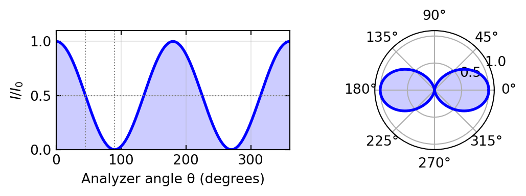
Consider linearly polarized light hitting a second polarizer (the analyzer) whose axis is rotated by \(\theta\). Only the field component along the analyzer axis passes, so the transmitted amplitude is \(E_0 \cos\theta\), and the intensity, being proportional to the amplitude squared, follows
\[I_{\text{transmitted}} = I_0 \cos^2(\theta) \tag{4}\]
This is Malus’s law. In Jones language: \(M(\theta)\,\mathbf{J}_H = \cos\theta \, \mathbf{J}_\theta\), whose squared norm is \(\cos^2\theta\). The dependence is plotted in Figure 2.
Stokes Parameters
The Jones formalism requires a fixed phase relation between \(E_x\) and \(E_y\), so it can only describe fully polarized light. Real light sources (the sun, lamps, LEDs) emit fields whose phase relation fluctuates on time scales far shorter than any detector can follow; such light is partially polarized or unpolarized. The Stokes parameters handle every case. They are built from time-averaged products of the field components, where \(\langle\,\cdot\,\rangle\) denotes the average over many optical cycles, which is what any detector measures:
\[S_0 = \langle E_x E_x^* \rangle + \langle E_y E_y^* \rangle \tag{5}\] \[S_1 = \langle E_x E_x^* \rangle - \langle E_y E_y^* \rangle\] \[S_2 = \langle E_x E_y^* + E_y E_x^* \rangle\] \[S_3 = i\langle E_y E_x^* - E_x E_y^* \rangle\]
Their physical meaning becomes obvious when each is written as a difference of two measurable intensities:
\[S_0 = I_H + I_V, \quad S_1 = I_H - I_V, \quad S_2 = I_{+45°} - I_{-45°}, \quad S_3 = I_{RCP} - I_{LCP}\]
\(S_0\) is the total intensity. \(S_1\) measures the preference for horizontal over vertical polarization, \(S_2\) the preference for \(+45°\) over \(-45°\), and \(S_3\) the preference for right over left circular. All four can be determined with nothing more than a polarizer, a quarter-wave plate, and a power meter; this is how polarization is measured in practice.
Examples
Unpolarized: \(\mathbf{S} = I_0 \begin{pmatrix} 1 \\ 0 \\ 0 \\ 0 \end{pmatrix}\), H-linear: \(\mathbf{S}_H = I_0 \begin{pmatrix} 1 \\ 1 \\ 0 \\ 0 \end{pmatrix}\), Right circular: \(\mathbf{S}_{RCP} = I_0 \begin{pmatrix} 1 \\ 0 \\ 0 \\ 1 \end{pmatrix}\)
For any beam, \(S_1^2 + S_2^2 + S_3^2 \leq S_0^2\), with equality exactly for fully polarized light. The degree of polarization
\[P = \frac{\sqrt{S_1^2 + S_2^2 + S_3^2}}{S_0}\]
interpolates between \(P = 0\) (unpolarized) and \(P = 1\) (fully polarized).
The Poincaré Sphere
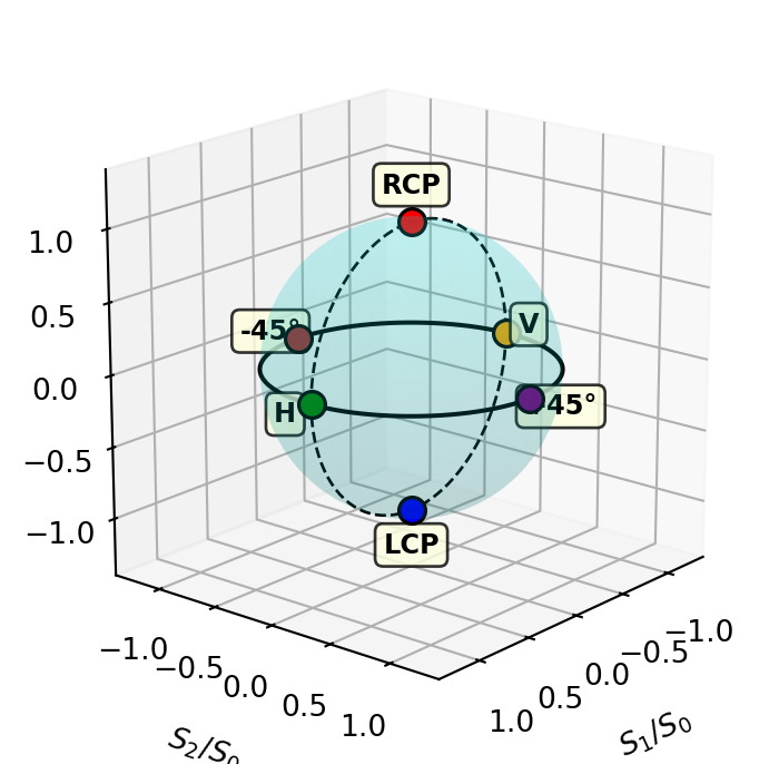
The Poincaré sphere turns the Stokes description into geometry. Using the normalized parameters
\[x = S_1/S_0, \quad y = S_2/S_0, \quad z = S_3/S_0,\]
every fully polarized state corresponds to one point on the unit sphere (\(P = 1\)), shown in Figure 3. The north pole is right circular, the south pole left circular, and the equator carries all linear polarizations; the rest of the surface represents elliptical states. Two diametrically opposite points are always orthogonal polarizations. Partially polarized light lies inside the sphere at radius \(P\), with unpolarized light at the center.
The sphere is more than a pretty picture: retarders rotate the sphere about the axis corresponding to their fast-axis polarization (by the angle \(\Gamma\)), and optical rotators rotate it about the polar axis. Any polarization transformation by lossless elements is simply a rotation of the sphere, which makes the design of polarization controllers remarkably intuitive.
Mueller Matrices
Just as Jones vectors transform by Jones matrices, Stokes vectors transform through optical elements via Mueller matrices (\(4 \times 4\), real). Their advantage is generality: they apply to partially polarized light and can describe depolarizing elements, which the Jones calculus cannot.
Horizontal polarizer: \[M_H = \frac{1}{2} \begin{pmatrix} 1 & 1 & 0 & 0 \\ 1 & 1 & 0 & 0 \\ 0 & 0 & 0 & 0 \\ 0 & 0 & 0 & 0 \end{pmatrix}\]
A quick payoff: applying \(M_H\) to unpolarized light \(\mathbf{S} = I_0(1, 0, 0, 0)^T\) gives \(\frac{I_0}{2}(1, 1, 0, 0)^T\). Half the intensity is transmitted, and the output is fully horizontally polarized, exactly as expected, and something no Jones vector could have expressed.
Retarder (retardance \(\Gamma\), fast axis horizontal): \[M_{\text{ret}} = \begin{pmatrix} 1 & 0 & 0 & 0 \\ 0 & 1 & 0 & 0 \\ 0 & 0 & \cos\Gamma & -\sin\Gamma \\ 0 & 0 & \sin\Gamma & \cos\Gamma \end{pmatrix}\]
This is the sphere rotation mentioned above: the retarder rotates the \((S_2, S_3)\) plane by \(\Gamma\) about the \(S_1\) axis. For \(\Gamma = \pi/2\) it maps \(+45°\) linear light, \(\mathbf{S} = I_0(1,0,1,0)^T\), to right circular, \(I_0(1,0,0,1)^T\), in agreement with the Jones worked example. (Sign conventions for \(S_3\) and \(\Gamma\) vary between books; the set used here is internally consistent with our definition of RCP.)
Practical Polarizing Elements
Linear Polarizers
A wire-grid polarizer consists of fine parallel metal wires. The field component parallel to the wires drives currents and is reflected, while the perpendicular component is transmitted. A dichroic sheet polarizer (Polaroid foil) contains aligned long-chain molecules that absorb one component; it is inexpensive and used in displays and sunglasses, but limited in damage threshold and extinction. The highest quality comes from birefringent crystal polarizers such as the Glan-Thompson prism: two cemented calcite prisms in which the unwanted polarization undergoes total internal reflection at the internal interface, achieving extinction ratios of \(10^{5}\) to \(10^{6}:1\).
Polarized light can also be produced by reflection alone: at the Brewster angle \(\theta_B = \arctan(n_2/n_1)\), the reflected beam contains no p-polarized component, so the reflection is perfectly s-polarized.
Retardance Plates
Wave plates are cut from birefringent crystals such as quartz, calcite, or mica, with ordinary and extraordinary indices \(n_o\) and \(n_e\). A plate of thickness \(d\) produces the retardance
\[\Gamma = \frac{2\pi\, \Delta n\, d}{\lambda}, \qquad \Delta n = |n_e - n_o| .\]
A quarter-wave plate (\(\Gamma = \pi/2\)) converts linear light at \(45°\) to its axes into circular light and vice versa; a half-wave plate (\(\Gamma = \pi\)) mirrors linear polarization about its fast axis and is the standard tool for rotating polarization. Because \(\Gamma\) depends on \(\lambda\), a simple wave plate works only near its design wavelength; achromatic retarders combine plates of different materials so that the wavelength dependence largely cancels.
Optical Rotation
Some materials rotate the plane of linear polarization as light propagates through them. In optically active (chiral) media such as sugar solutions or quartz, the rotation angle grows linearly with path length, \(\theta = \alpha \ell\), with the rotatory power \(\alpha\). In Faraday rotation, a longitudinal magnetic field induces the rotation \(\theta = V B \ell\), with the Verdet constant \(V\). Faraday rotation is non-reciprocal: the sense of rotation does not reverse when the light direction reverses. This property is the basis of optical isolators, the one-way valves of laser optics.
Summary
Polarization is the oscillation direction of the electric field perpendicular to propagation; it is fixed by two amplitudes and the relative phase \(\delta\).
Three states: linear (straight oscillation), circular (rotation at constant magnitude), elliptical (the general case).
Jones vectors/matrices describe fully polarized light; Stokes parameters/Mueller matrices describe any state, including partially polarized light.
Poincaré sphere: geometric representation of all polarization states; lossless elements act as rotations of the sphere.
Optical elements: polarizers (project onto an axis), retarders (delay one axis by \(\Gamma\)), rotators (turn the polarization plane).
Key applications: fiber optics, LCD displays, stress analysis, quantum optics.
The chain from Maxwell’s equations through the Jones calculus to the Poincaré sphere shows how a small set of linear-algebra tools captures the entire subject.
Experimental Connections
Polarization is one of the most accessible optical phenomena for hands-on experiments. The following activities connect the theory above to real laboratory practice:
Polarizer and analyzer (Malus’s law) Set up two linear polarizers on an optical rail with a white-light source or laser. Rotate the analyzer in 10° steps and measure the transmitted intensity with a photodetector. Plot \(I(\theta)\) and fit to \(I_0 \cos^2\theta\). Deviations from perfect extinction reveal the quality of your polarizers and any residual birefringence in optical components.
Quarter-wave plate: linear to circular Insert a quarter-wave plate between crossed polarizers. Rotate it until the fast axis is at 45° to the first polarizer, and you recover maximum transmission through the analyzer (since circular polarization has equal projections on any linear axis). Verify by rotating the analyzer: the intensity should be nearly constant.
Stress birefringence (photoelasticity) Place a transparent plastic ruler or protractor between crossed polarizers and illuminate with white light. The colorful fringe patterns reveal internal stress from the manufacturing process. This directly visualizes how mechanical stress creates birefringence. Quantitative analysis connects stress to the retardance via the stress-optic coefficient.
Optical activity in sugar solutions Fill a glass tube with sugar solution of known concentration. Place between crossed polarizers and observe the rotation of the polarization plane. By varying concentration and tube length, verify the linear dependence \(\theta = [\alpha] \cdot c \cdot L\). This is the basis of saccharimetry (sugar concentration measurement in the food industry).
Brewster angle measurement Reflect a laser beam off a glass surface (microscope slide) and vary the angle of incidence. At Brewster’s angle \(\theta_B = \arctan(n)\), the reflected beam is perfectly linearly polarized. Verify with a polarizer. This gives an elegant measurement of the refractive index.
Further Reading
The following references are linked to the central Resources & Recommended Reading page:
- Saleh & Teich, Ch. 6: Polarization Optics. Systematic development of Jones and Mueller calculus with many worked examples.
- Hecht, Ch. 8: Polarization. Excellent physical intuition, many photographs of real polarization effects.
- Goldstein (2011): Polarized Light. Comprehensive reference for Stokes parameters, Mueller matrices, and the Poincaré sphere.
- Collett (2005): Field Guide to Polarization. Compact summary of all key formulae.
- Born & Wolf, Ch. 1, 14–15: Rigorous EM treatment of polarization and crystal optics.
Introduction to Photonics: Polarization of Light