Theories for light

Matrix Optics

The linear relation between input and output parameters allows us to express optical elements as linear transformations (matrices). This approach forms the foundation of matrix optics. For a lens, the matrix representation is:

\[\begin{pmatrix} y_2 \\ \theta_2 \end{pmatrix} = \begin{pmatrix} 1 & 0 \\ -\frac{1}{f} & 1 \end{pmatrix} \begin{pmatrix} y_1 \\ \theta_1 \end{pmatrix}\]

This 2×2 matrix is called the ABCD matrix of the lens. Thanks to the linearization of Snell’s law, we can generalize this to any optical element:

\[\begin{pmatrix} y_2 \\ \theta_2 \end{pmatrix} = \begin{pmatrix} A & B \\ C & D \end{pmatrix} \begin{pmatrix} y_1 \\ \theta_1 \end{pmatrix}\]

Each element in the ABCD matrix has a specific physical meaning:

Matrix Element	Physical Meaning
A	Magnification - relates output position to input position
B	Position-to-angle conversion - relates output position to input angle
C	Focusing power - relates output angle to input position
D	Angular magnification - relates output angle to input angle

Every optical element can be characterized by these parameters. For example, a lens has C = -1/f (focusing power), while free space has B = d (position-dependent angle change). An important property is that the determinant of the matrix equals the ratio of refractive indices: det(M) = n₁/n₂, which equals 1 in a single medium.

Here are the ABCD matrices for common optical elements:

\[ \mathbf{M}=\begin{bmatrix} A & B\\ C & D \end{bmatrix} =\left[\begin{array}{ll} 1 & d \\ 0 & 1 \end{array}\right] \tag{Free space} \]

\[ \mathbf{M}=\left[\begin{array}{cc} 1 & 0 \\ 0 & \frac{n_1}{n_2} \end{array}\right] \tag{Planar interface} \]

\[ \mathbf{M}=\left[\begin{array}{cc} 1 & 0 \\ -\frac{\left(n_2-n_1\right)}{n_2 R} & \frac{n_1}{n_2} \end{array}\right] \tag{Spherical Boundary} \]

\[ \mathbf{M}=\left[\begin{array}{cc} 1 & 0 \\ -\frac{1}{f} & 1 \end{array}\right] \tag{Thin Lens} \]

For a system containing multiple optical elements, we simply multiply their matrices in the order that light passes through them:

\[ \mathrm{M}=\mathbf{M}_N \cdots \mathbf{M}_2 \mathbf{M}_1 \]

A ray entering the first optical element at a height \(y_1\) at an angle \(\theta_1\) is transformed according to the matrix \(\mathbf{M}\) by the whole system. This elegant approach provides a powerful tool for analyzing complex optical systems efficiently.

Example: Optical Cloaking with Lens Systems

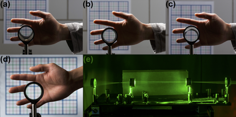
Optical cloaking refers to making objects “invisible” by guiding light rays around them such that to an observer, it appears as if the rays traveled through free space without encountering any object. Using matrix optics, we can design such a system.

Figure 1— Example of a practical paraxial cloak. (a)–(c) A hand is cloaked for varying directions, while the background image is transmitted properly.(d) On-axis view of the ray optics cloaking device. (e) Setup using practical, easy to obtain optics, for demonstrating paraxial cloaking principles. (Photos by J. Adam Fenster, videos by Matthew Mann / University of Rochester) Source

For perfect optical cloaking, the ABCD matrix of our system must be equivalent to that of free space:

\[ \mathbf{M}_{cloaking} = \left[\begin{array}{cc} 1 & d \\ 0 & 1 \end{array}\right] \]

Where \(d\) is the total effective optical path length. Let’s explore why we need exactly 4 lenses to achieve this.

Analysis of Different Lens Configurations

1. Single Lens Configuration

For a single lens with focal length \(f\), the ABCD matrix is:

\[ \mathbf{M}_{single} = \left[\begin{array}{cc} 1 & 0 \\ -\frac{1}{f} & 1 \end{array}\right] \]

This clearly cannot match the free space matrix due to the non-zero \(C\) element.

2. Two-Lens Configuration

For two lenses with focal lengths \(f_1\) and \(f_2\) separated by distance \(d_{12}\):

\[ \mathbf{M}_{two} = \left[\begin{array}{cc} 1 & 0 \\ -\frac{1}{f_2} & 1 \end{array}\right] \left[\begin{array}{cc} 1 & d_{12} \\ 0 & 1 \end{array}\right] \left[\begin{array}{cc} 1 & 0 \\ -\frac{1}{f_1} & 1 \end{array}\right] \]

When \(d_{12} = f_1 + f_2\) (telescopic arrangement), this simplifies to:

\[ \mathbf{M}_{two} = \left[\begin{array}{cc} -\frac{f_1}{f_2} & 0 \\ 0 & -\frac{f_2}{f_1} \end{array}\right] \]

Since both magnification (\(A\)) and angular magnification (\(D\)) cannot simultaneously equal 1 while maintaining \(\det(\mathbf{M}) = 1\), two lenses are insufficient.

3. Three-Lens Configuration

With three lenses, we have more parameters but still need to determine if we can satisfy all constraints simultaneously. For a three-lens system with focal lengths \(f_1\), \(f_2\), and \(f_3\), separated by distances \(d_{12}\) and \(d_{23}\), the system matrix would be:

\[ \mathbf{M}_{three} = \left[\begin{array}{cc} 1 & 0 \\ -\frac{1}{f_3} & 1 \end{array}\right] \left[\begin{array}{cc} 1 & d_{23} \\ 0 & 1 \end{array}\right] \left[\begin{array}{cc} 1 & 0 \\ -\frac{1}{f_2} & 1 \end{array}\right] \left[\begin{array}{cc} 1 & d_{12} \\ 0 & 1 \end{array}\right] \left[\begin{array}{cc} 1 & 0 \\ -\frac{1}{f_1} & 1 \end{array}\right] \]

When multiplied out, the focusing power (C element) of the system is:

\[C = -\frac{1}{f_3} - \frac{1}{f_2} - \frac{1}{f_1} + \frac{d_{12}}{f_1f_2} + \frac{d_{23}}{f_2f_3} + \frac{d_{12}d_{23}}{f_1f_2f_3}\]

The magnification (A element) of the system is:

\[A = 1 - \frac{d_{12}}{f_1} - \frac{d_{23}}{f_2} + \frac{d_{12}d_{23}}{f_1f_2}\]

For perfect cloaking, we need both C = 0 and A = 1. From A = 1, we can derive:

\[\frac{d_{12}}{f_1} + \frac{d_{23}}{f_2} - \frac{d_{12}d_{23}}{f_1f_2} = 0\]

Solving for \(d_{23}\), we get:

\[d_{23} = \frac{d_{12}/f_1}{1/f_2 - d_{12}/(f_1f_2)}\]

Substituting this into the condition for C = 0, we obtain a complex expression that places constraints on the possible values of \(f_1\), \(f_2\), and \(f_3\). For typical lens configurations, this results in values that are difficult to realize physically, as it often requires either negative separations or negative focal lengths.

While the three-lens system provides more parameters to work with than the two-lens system, the mathematical constraints of simultaneously achieving zero focusing power (C = 0) and unit magnification (A = 1) still make perfect cloaking challenging with conventional optical elements.

4. Four-Lens Configuration: The Solution

We can arrange four lenses in two pairs:

• First pair (lenses 1 and 2): A beam compressor
• Second pair (lenses 3 and 4): A beam expander

For the beam compressor (large lens \(f_1\) first, small lens \(f_2\) second), the two lenses must be separated by \(f_1+f_2\) to form a telescope. Multiplying the three matrices — lens, free space, lens — gives:

\[ \mathbf{M}_{comp} = \left[\begin{array}{cc} -\frac{f_2}{f_1} & f_1+f_2 \\ 0 & -\frac{f_1}{f_2} \end{array}\right] \]

The \(A\) element \(-f_2/f_1 < 1\) compresses the beam height; the \(D\) element \(-f_1/f_2\) increases the angle. Crucially, \(B = f_1+f_2 \neq 0\): the compressor is not equivalent to free space on its own.

The beam expander is the compressor in reverse (\(f_3 = f_2\) first, \(f_4 = f_1\) second, separation \(f_3+f_4 = f_1+f_2\)):

\[ \mathbf{M}_{exp} = \left[\begin{array}{cc} -\frac{f_1}{f_2} & f_1+f_2 \\ 0 & -\frac{f_2}{f_1} \end{array}\right] \]

Now place a free-space gap \(d_0\) between the two pairs. The full system matrix is \(\mathbf{M}_{exp}\cdot\mathbf{M}_{d_0}\cdot\mathbf{M}_{comp}\), which works out to:

\[ \mathbf{M}_{total} = \left[\begin{array}{cc} 1 & d_0\!\left(\dfrac{f_1}{f_2}\right)^{\!2} - \dfrac{2f_1(f_1+f_2)}{f_2} \\ 0 & 1 \end{array}\right] \]

This is exactly the free-space matrix with effective length \(d_{\mathrm{eff}}\), provided:

\[ d_{\mathrm{eff}} = d_0\!\left(\frac{f_1}{f_2}\right)^{\!2} - \frac{2f_1(f_1+f_2)}{f_2} > 0 \quad\Longrightarrow\quad d_0 > \frac{2f_2(f_1+f_2)}{f_1} \]

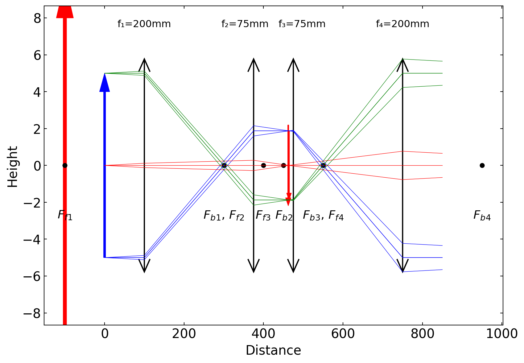
For \(f_1=200\,\mathrm{mm}\), \(f_2=75\,\mathrm{mm}\): \(d_{0,\min} \approx 206\,\mathrm{mm}\). The cloaking region \(d_{\mathrm{eff}}\) is the space between the two inner lenses that an object can occupy while remaining invisible — any ray traversing it exits the system as if it had traveled \(d_{\mathrm{eff}}\) of free space.

\[ \mathbf{M}_{cloaking} = \left[\begin{array}{cc} 1 & d_{\mathrm{eff}} \\ 0 & 1 \end{array}\right] \]

# Example of optical cloaking with four lenses using raytracing
from raytracing import *

# Define focal lengths (in mm)
f1 = 200
f2 = 75
f3 = f2  # f3 = f2 = 75
f4 = f1  # f4 = f1 = 200

# Create an optical path
path = OpticalPath()

# Add the four lenses with proper spacing
path.append(Space(d=100))  # Initial space before first lens
path.append(Lens(f=f1, label=f"f₁={f1}mm"))
path.append(Space(d=f1+f2))  # Distance between lens 1 and 2 (compressor)
path.append(Lens(f=f2, label=f"f₂={f2}mm"))
path.append(Space(d=100))  # Gap d₀ between lens pairs
path.append(Lens(f=f3, label=f"f₃={f3}mm"))
path.append(Space(d=f3+f4))  # Distance between lens 3 and 4 (expander)
path.append(Lens(f=f4, label=f"f₄={f4}mm"))
path.append(Space(d=100))  # Final space after last lens

# Display the ray path with custom figure size

path.display(
    raysList=[
        [Ray(y=5, theta=0)],
        [Ray(y=-5, theta=0)]
    ],
    interactive=False,
    limitObjectToFieldOfView=False,
    onlyPrincipalAndAxialRays=False
)

Multifocal Imaging

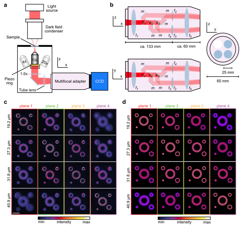
We would like to explore the concept of multifocal imaging to obtain 3D resolution from a single image. In a microscope, an objective lens together with a tube lens is used to focus light from a sample onto a detector. Either the tube lens is no modified to shift the focal plane of the objective lens or one uses multiple tube lenses with different focal lengths with a single objective lens.

Figure 2— The multifocal adapter. (a) Composition of the multifocal imaging setup. The multifocal adapter (MFA) is inserted into the light path between a standard dark-field microscope and a camera. (b) Composition of the multifocal adapter. Incoming light from the microscope is infinity projected by the lens f1 and split by three consecutive beam-splitters (b1 = 25/75; b2 = 33/67; b3 = 50/50). Five mirrors (m) guide the light into four separate optical paths. The lens f5 projects the four images onto the camera chip. The inter-plane distance is set by lenses of different focal length (f1 - f4). (c, d) Experimentally acquired (c) and simulated (d) (see Methods) multifocal dark-field images (planes 1 - 4, 20x objective) of a calibration grid at the four focal positions (indicated on the left side), where one of the four focal planes maps the grid sharply. Scale bar represents 20 µm. Experiment was performed six times with similar results. Source

In the simplest configuration of an objective lens and a tube lens, the light first travels from the object to the objective lens in free space for a distance \(s\), which is represented by

\[ M_1=\left[\begin{matrix}1 & s\\0 & 1\end{matrix}\right] \]

Then it is passing the objective lens with

\[ M_2=\left[\begin{matrix}1 & 0\\- \frac{1}{f_{1}} & 1\end{matrix}\right] \]

traveling further through free space with distance \(d\)

\[ M_3=\left[\begin{matrix}1 & d\\0 & 1\end{matrix}\right] \]

and then hitting the tube lens with

\[ M_4=\left[\begin{matrix}1 & 0\\- \frac{1}{\Delta_{ft} + f_{t}} & 1\end{matrix}\right] \]

where \(\Delta_ft\) is a parameter modifying the original tube lens focal distance \(f_t\). Finally, the light will propagate to the detector at distance \(f_t\) from the tube lens

\[ M_s=\left[\begin{matrix}1 & f_{t}\\0 & 1\end{matrix}\right] \]

giving for the whole system:

\[ M_t=M_4 M_3 M_2 M_1 \]

The final matrix has again 4 parameters \(A,B,C\) and \(D\). For sharp imaging the parameter \(B\) of the system must be equal to zero, as the outgoing light should be independent of the incoming angle. This is achieved

\[\delta s=\frac{f_{1} \left(\Delta_{ft} d + \Delta_{ft} f_{t} + f_{t}^{2}\right)}{\Delta_{ft} d - \Delta_{ft} f_{1} + \Delta_{ft} f_{t} + f_{t}^{2}}-s_0 \]

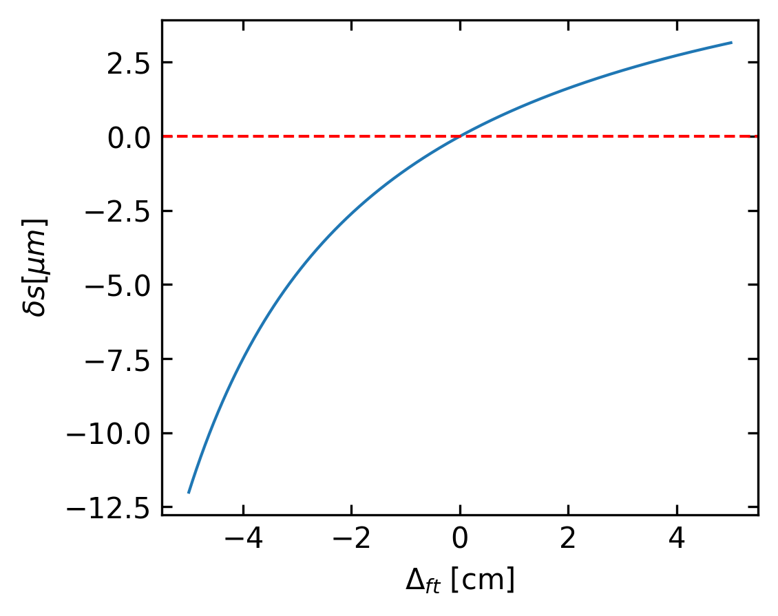
Figure 3— Required object-plane shift \(\delta s\) (in µm) to restore sharp imaging (\(B=0\)) as a function of tube-lens focal-length detuning \(\Delta_{ft}\) for a two-lens microscope with objective focal length \(f_1 = 0.18\,\text{cm}\), nominal tube-lens focal length \(f_t = 18\,\text{cm}\), and objective-to-tube-lens separation \(d = 20\,\text{cm}\). A positive detuning of the tube lens forces the object to be moved closer to the objective to re-establish the imaging condition.

The B Parameter

The B parameter is the most direct indicator of a sharp image in matrix optics. For an optical system with ABCD matrix: \[ \begin{pmatrix} y_2 \\ \theta_2 \end{pmatrix} = \begin{pmatrix} A & B \\ C & D \end{pmatrix} \begin{pmatrix} y_1 \\ \theta_1 \end{pmatrix} \]

The output position is given by: \[y_2 = Ay_1 + B\theta_1\]

For an image to be sharp, all rays originating from the same object point must converge to a single image point, regardless of their initial angles. This means that for a given \(y_1\) (object position), the final position \(y_2\) must be independent of the initial angle \(\theta_1\).

This condition is satisfied when B = 0.

When B = 0: - The final position depends only on the initial position (\(y_2 = Ay_1\)) - All rays from a point source converge to a single point in the image plane - The imaging is “stigmatic” (point-to-point mapping)

In our lens example, the system matrix was: \[ \mathbf{M}_{system} = \left[\begin{array}{cc} 1-\frac{d}{f} & d \\ -\frac{1}{f} & 1 \end{array}\right] \]

For parallel input rays (different \(y_1\) but all \(\theta_1 = 0\)), we needed A = 0 to make them all converge to a single point, which happened when d = f.

But for general imaging of points (not just parallel rays), the B = 0 condition is what determines whether the image is sharp. This is why, in optical design, finding conjugate planes (where B = 0) is essential for sharp imaging.

Application: Autofocus by Beam Displacement

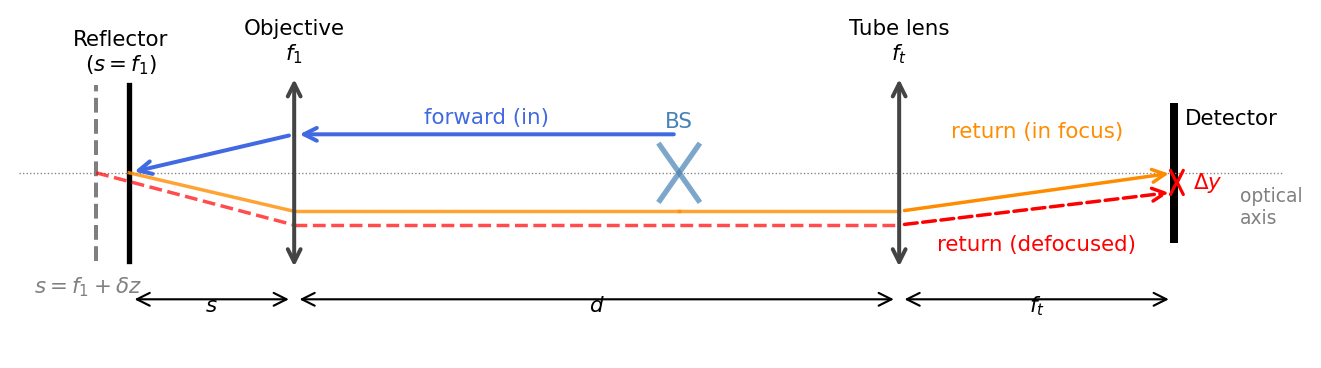
Modern microscopes often incorporate a reflection-based autofocus system. The idea is elegant: an auxiliary light beam, launched off-axis but parallel to the optical axis, is coupled into the infinity space between objective and tube lens via a beam splitter. This beam travels through the objective, reflects off a refractive-index boundary near the sample plane (e.g. the cover-glass surface), returns through the objective, and is detected on the camera. A shift of the reflecting surface along the optical axis produces a measurable lateral displacement of the return beam on the detector, providing a focus-error signal without any mechanical scanning.

We can analyse this system entirely with the ABCD matrix formalism using the same parameters as before.

Unfolded Round-Trip

Because the reflector is flat and perpendicular to the optical axis, the round-trip can be “unfolded” into a single straight optical path. The beam starts at the beam-splitter position (distance \(d\) from the objective), propagates to the objective, passes through it, travels a distance \(s\) to the reflecting surface, continues (unfolded) another distance \(s\) back through the objective, traverses the infinity space back to the tube lens, and finally propagates to the camera.

The complete matrix for this path is

\[ M_\mathrm{AF} = \underbrace{M_\mathrm{camera}}_{\text{tube lens}\to\text{detector}}\;\underbrace{M_\mathrm{return}}_{\text{sample}\to\text{BS}}\;\underbrace{M_\mathrm{forward}}_{\text{BS}\to\text{sample}} \]

with the three blocks

\[ M_\mathrm{forward} = \begin{pmatrix}1 & s\\0 & 1\end{pmatrix}\begin{pmatrix}1 & 0\\-1/f_1 & 1\end{pmatrix}\begin{pmatrix}1 & d\\0 & 1\end{pmatrix}, \qquad M_\mathrm{return} = \begin{pmatrix}1 & d\\0 & 1\end{pmatrix}\begin{pmatrix}1 & 0\\-1/f_1 & 1\end{pmatrix}\begin{pmatrix}1 & s\\0 & 1\end{pmatrix} \]

\[ M_\mathrm{camera} = \begin{pmatrix}1 & f_t\\0 & 1\end{pmatrix}\begin{pmatrix}1 & 0\\-1/f_t & 1\end{pmatrix} \]

The input ray is \((y_\mathrm{in},\,\theta_\mathrm{in}) = (h,\,0)\), i.e. off-axis by height \(h\), but parallel to the axis. The lateral position on the camera is then simply \(y_\mathrm{cam} = A_\mathrm{AF}\, h\), where \(A_\mathrm{AF}\) is the (1,1) element of \(M_\mathrm{AF}\).

Figure 4— Schematic of the reflection-based autofocus beam path. An off-axis beam (blue) enters the infinity space via a beam splitter, is focused by the objective onto the reflecting surface, and returns (red/orange) through the objective and tube lens to the camera. When the reflector is displaced by \(\delta z\) from the focal plane (dashed), the return beam arrives at a shifted lateral position \(\Delta y\) on the detector.

The full system matrix is

\[ M_\mathrm{AF} = \left[\begin{matrix}\frac{2 f_{t} \left(- f_{1} + s\right)}{f_{1}^{2}} & \frac{f_{t} \left(- d \left(f_{1} - s\right) - f_{1} s - \left(d - f_{1}\right) \left(f_{1} - s\right)\right)}{f_{1}^{2}}\\\frac{d f_{1} - f_{1} f_{t} + f_{t} s - s \left(d - f_{1}\right) + \left(f_{1} - s\right) \left(d - f_{1} - f_{t}\right)}{f_{1}^{2} f_{t}} & \frac{\left(d - f_{1}\right) \left(d f_{1} - f_{1} f_{t} + f_{t} s - s \left(d - f_{1}\right)\right) + \left(d \left(f_{1} - s\right) + f_{1} s\right) \left(d - f_{1} - f_{t}\right)}{f_{1}^{2} f_{t}}\end{matrix}\right] \]

The detector-plane position of the return beam is

\[ y_\mathrm{cam}(s) = A_\mathrm{AF}(s)\cdot h \]

and the autofocus signal, i.e. the lateral displacement relative to the in-focus position \(s_0 = f_1\), is

\[ \Delta y(s) = y_\mathrm{cam}(s) - y_\mathrm{cam}(f_1). \]

At perfect focus (\(s = f_1\)) the A element simplifies to

\[ A_\mathrm{AF}(f_1) = 0 \]

Numerical Example

We use the same microscope parameters as for the focal-shift calculation: \(f_1 = 0.18\;\text{cm}\) (100× objective), \(f_t = 18\;\text{cm}\), \(d = 20\;\text{cm}\), and an input beam height \(h = 0.5\;\text{cm}\).

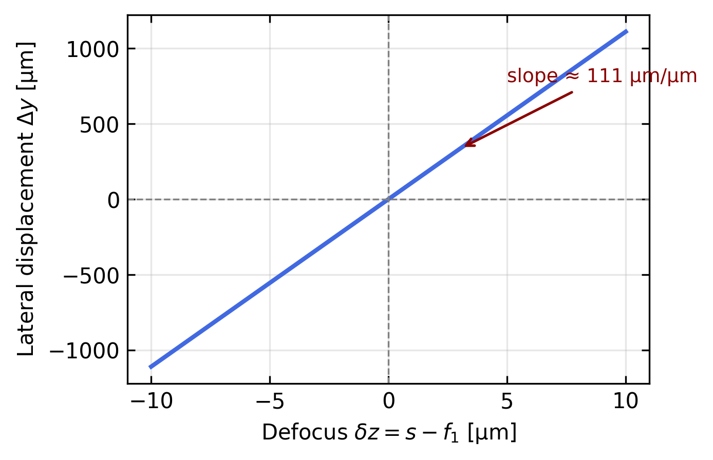
Figure 5— Reflection-based autofocus: lateral beam displacement \(\Delta y\) on the camera as a function of the defocus \(\delta z = s - f_1\). Parameters: \(f_1 = 0.18\,\text{cm}\) (100× objective), \(f_t = 18\,\text{cm}\), \(d = 20\,\text{cm}\), \(h = 0.1\,\text{cm}\). The linear slope provides a sensitive focus-error signal whose sign indicates the direction of the defocus.

The plot confirms that the lateral beam displacement on the camera is a perfectly linear function of the defocus, a direct consequence of the ABCD matrix element \(A_\mathrm{AF} = 2 f_t\,(s - f_1)/f_1^2\). The sensitivity is set by the slope

\[ \frac{\Delta y}{\delta z} = \frac{2\,M\,h}{f_1} \]

where \(M = f_t/f_1\) is the magnification of the objective–tube-lens pair. For a 100× objective with \(h = 1\;\text{mm}\), this gives \({\sim}\,111\;\text{µm}/\text{µm}\). A sample displacement of just 1 µm produces a beam shift of over 100 µm on the camera, easily detectable with a position-sensitive detector or a split photodiode.

Practical Autofocus Implementation

In a real microscope autofocus system (such as the Nikon Perfect Focus or Olympus Z-drift compensator):

• The auxiliary beam uses an infrared LED (\(\lambda \approx 870\;\text{nm}\)) to avoid interfering with fluorescence imaging.
• A split photodiode or quadrant detector measures the lateral displacement and feeds back to a piezo z-stage in a closed-loop control.
• The reflecting interface is typically the cover-glass–medium boundary or a dedicated reference surface.
• The system operates continuously, correcting thermal drift and mechanical vibrations at rates of several hundred Hz.