lecture01 – Photonics

Theories for light

Light has been described through increasingly sophisticated theoretical frameworks throughout the history of physics. The simplest framework is Ray Optics or Geometrical Optics, which treats light as rays traveling along straight paths and applies geometrical principles to describe interactions with optical elements like lenses and mirrors. Moving beyond this approximation, Wave Optics introduces the wave nature of light, explaining phenomena such as interference and diffraction that ray optics cannot address. Electromagnetic Optics further refines our understanding by treating light as electromagnetic waves governed by Maxwell’s equations, providing a complete classical description of light-matter interactions. For intense light sources, Nonlinear Optics becomes essential, describing how materials respond nonlinearly to strong electromagnetic fields, giving rise to frequency conversion and other novel effects. Finally, at the most fundamental level, Quantum Optics treats light as consisting of photons—quantum mechanical particles exhibiting both wave and particle properties—essential for understanding phenomena like spontaneous emission, entanglement, and the quantum nature of light-matter interactions. This course will progressively build your understanding through these increasingly sophisticated frameworks.

Ray Optics

Ray optics, or geometric optics, provides a powerful framework for understanding light propagation when the wavelength is much smaller than the dimensions of optical elements involved. In this approach, light travels along straight lines called rays in homogeneous media, with well-defined paths that can be mathematically traced. This description serves as the foundation for analyzing many optical systems, from simple mirrors to complex microscopes and telescopes.

Fermat’s Principle: Integral and Differential Forms

Fermat’s Principle forms one of the foundations of ray optics, stating that light travels along the route that takes the total optical path length between any two points to an extremum (commonly a minimum). This optical path length, expressed mathematically as \(\int_C n(s)ds\), represents the effective distance light traverses through media of varying refractive indices. When this quantity is divided by the vacuum speed of light \(c_0\), it yields the total travel time required for light to journey between those points.

In its integral form:

\[\delta\int_C n(s)ds = 0\]

where \(n(s)\) is the refractive index along path \(C\) and \(ds\) is the differential path length.

The same principle can be expressed as a differential equation that describes how light bends in media with varying refractive indices:

\[\frac{d}{ds}\left(n\frac{d\mathbf{r}}{ds}\right) = \nabla n\]

This equation shows that rays bend toward regions of higher refractive index. In homogeneous media (\(\nabla n = 0\)), it simplifies to \(\frac{d^2\mathbf{r}}{ds^2} = 0\), confirming that light follows straight lines.

Optical Laws Derived from Fermat’s Principle

Reflection: At a planar interface, Fermat’s Principle directly yields the law of reflection:

\[\theta_i = \theta_r\]

where \(\theta_i\) is the angle of incidence and \(\theta_r\) is the angle of reflection, both measured from the normal to the surface.

Code

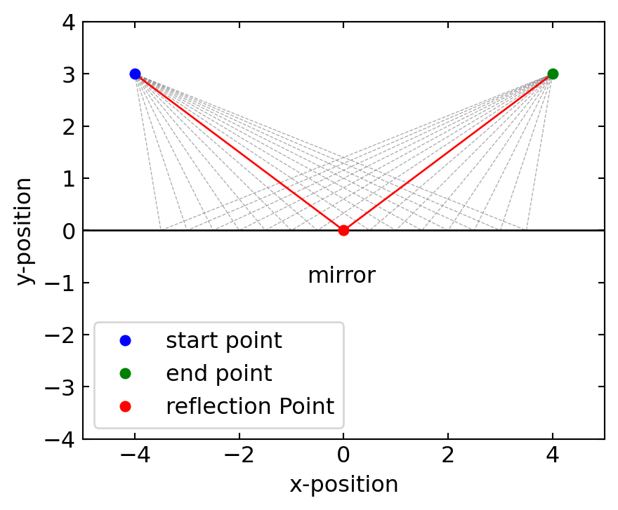
def calculate_path_length(x, start, end):
    """Calculate the total path length from start to point x to end"""
    d1 = np.sqrt((x - start[0])**2 + (start[1])**2)
    d2 = np.sqrt((end[0] - x)**2 + (end[1])**2)
    return d1 + d2

# Set up the figure
fig, ax = plt.subplots(figsize=get_size(15, 10))

# Define start and end points
start_point = (-4, 3)
end_point = (4, 3)

# X positions for different possible paths
x_positions = np.linspace(-3.5, 3.5, 15)

# Calculate path lengths
path_lengths = [calculate_path_length(x, start_point, end_point) for x in x_positions]

# Find the minimum path (Fermat's principle)
min_index = np.argmin(path_lengths)
min_x = x_positions[min_index]

# Plot the horizontal line (interface)
ax.axhline(y=0, color='black', linestyle='-', linewidth=1)

# Plot all possible paths
for i, x in enumerate(x_positions):
    if i == min_index:
        continue  # Skip the minimum path for now

    # Create path
    verts = [
        start_point,
        (x, 0),
        end_point
    ]
    codes = [
        Path.MOVETO,
        Path.LINETO,
        Path.LINETO
    ]
    path = Path(verts, codes)
    patch = patches.PathPatch(path, facecolor='none', edgecolor='gray',
                             linestyle='--', lw=0.5,alpha=0.65)
    ax.add_patch(patch)

# Plot the minimum path (Fermat's Principle)
verts = [
    start_point,
    (min_x, 0),
    end_point
]
codes = [
    Path.MOVETO,
    Path.LINETO,
    Path.LINETO
]
path = Path(verts, codes)
patch = patches.PathPatch(path, facecolor='none', edgecolor='red',
                         linestyle='-')
ax.add_patch(patch)

# Add dots for the points
ax.plot(start_point[0], start_point[1], 'bo', label='start point')
ax.plot(end_point[0], end_point[1], 'go',  label='end point')
ax.plot(min_x, 0, 'ro',  label='reflection Point')

# Set labels and title
ax.set_xlabel('x-position')
ax.set_ylabel('y-position')
ax.text(-0.7, -1, "mirror")

# Set plot limits and legend
ax.set_xlim(-5, 5)
ax.set_ylim(-4, 4)
ax.set_aspect('equal')
ax.legend()

plt.tight_layout()
plt.show()

Figure 1— Fermat’s principle for reflection of light at an interface

Reflection Law Derivation

For reflection at a planar interface, we consider a ray traveling from point A to point B via reflection at point P on a mirror, as illustrated in Fig. \(\ref{fig-fermat-reflection}\). The total path length is \(L = |AP| + |PB|\).

Let’s establish a coordinate system where the mirror lies along the x-axis at y = 0. If point A is at coordinates \((-a, h_1)\) and point B is at \((b, h_2)\), with the reflection point P at \((x, 0)\), the total path length is:

\[L(x) = \sqrt{(x+a)^2 + h_1^2} + \sqrt{(b-x)^2 + h_2^2}\]

According to Fermat’s Principle, the actual path minimizes \(L\), so we differentiate with respect to \(x\) and set it equal to zero:

\[\frac{dL}{dx} = \frac{x+a}{\sqrt{(x+a)^2 + h_1^2}} - \frac{b-x}{\sqrt{(b-x)^2 + h_2^2}} = 0\]

Rearranging this equation:

\[\frac{x+a}{\sqrt{(x+a)^2 + h_1^2}} = \frac{b-x}{\sqrt{(b-x)^2 + h_2^2}}\]

Now, let’s interpret this geometrically. The angle of incidence \(\theta_i\) is the angle between the incident ray AP and the normal to the mirror (y-axis). Similarly, the angle of reflection \(\theta_r\) is the angle between the reflected ray PB and the normal.

From trigonometry:

\(\sin(\theta_i) = \frac{x+a}{\sqrt{(x+a)^2 + h_1^2}}\)
\(\sin(\theta_r) = \frac{b-x}{\sqrt{(b-x)^2 + h_2^2}}\)

Therefore, our minimization condition directly yields: \[\sin(\theta_i) = \sin(\theta_r)\]

Since both angles are measured in the same quadrant (from the normal to the mirror), this equality implies: \[\theta_i = \theta_r\]

This is the law of reflection: the angle of incidence equals the angle of reflection.

Law of Reflection: The angle of incidence equals the angle of reflection. \[\theta_i = \theta_r\]

Refraction: Between media with different refractive indices, Fermat’s Principle yields Snell’s law:

\[n_1\sin\theta_1 = n_2\sin\theta_2\]

where \(\theta_1\) and \(\theta_2\) are the angles of incidence and refraction, respectively.

Code

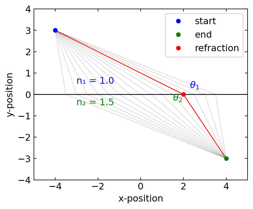
def calculate_optical_path(x, start, end, n1, n2):
    """Calculate the total optical path length from start to point x to end"""
    d1 = n1 * np.sqrt((x - start[0])**2 + (start[1])**2)  # Optical path in medium 1
    d2 = n2 * np.sqrt((end[0] - x)**2 + (end[1])**2)      # Optical path in medium 2
    return d1 + d2

# Set up the figure
fig, ax = plt.subplots(figsize=get_size(15, 10))

# Define start and end points
start_point = (-4, 3)
end_point = (4, -3)

# Define refractive indices
n1 = 1.0  # Medium 1 (above interface)
n2 = 1.5  # Medium 2 (below interface)

# X positions for different possible paths
x_positions = np.linspace(-3.5, 3.5, 15)

# Calculate optical path lengths
optical_paths = [calculate_optical_path(x, start_point, end_point, n1, n2) for x in x_positions]

# Find the minimum path (Fermat's principle)
min_index = np.argmin(optical_paths)
min_x = x_positions[min_index]

# Plot the horizontal line (interface)
ax.axhline(y=0, color='black', linestyle='-', linewidth=1)

# Plot all possible paths
for i, x in enumerate(x_positions):
    if i == min_index:
        continue  # Skip the minimum path for now

    # Create path
    verts = [
        start_point,
        (x, 0),
        end_point
    ]
    codes = [
        Path.MOVETO,
        Path.LINETO,
        Path.LINETO
    ]
    path = Path(verts, codes)
    patch = patches.PathPatch(path, facecolor='none', edgecolor='gray',
                             linestyle='--', lw=0.5, alpha=0.65)
    ax.add_patch(patch)

# Plot the minimum path (Fermat's Principle)
verts = [
    start_point,
    (min_x, 0),
    end_point
]
codes = [
    Path.MOVETO,
    Path.LINETO,
    Path.LINETO
]
path = Path(verts, codes)
patch = patches.PathPatch(path, facecolor='none', edgecolor='red',
                         linestyle='-', lw=1)
ax.add_patch(patch)

# Add dots for the points
ax.plot(start_point[0], start_point[1], 'bo', label='start')
ax.plot(end_point[0], end_point[1], 'go', label='end')
ax.plot(min_x, 0, 'ro', label='refraction')

# Calculate and draw angles
# Incident ray
dx1 = min_x - start_point[0]
dy1 = 0 - start_point[1]
incident_angle = np.arctan2(-dy1, dx1)
theta1 = np.pi/2 - incident_angle

# Refracted ray
dx2 = end_point[0] - min_x
dy2 = end_point[1] - 0
refracted_angle = np.arctan2(dy2, dx2)
theta2 = np.pi/2 + refracted_angle

# Draw angle arcs

# Add angle labels
ax.text(min_x + 0.3, 0.3, r'$\theta_1$', color='blue')
ax.text(min_x - 0.5, -0.3, r'$\theta_2$', color='green')

# Set labels and title
ax.set_xlabel('x-position')
ax.set_ylabel('y-position')
ax.text(-3, 0.5, f"n₁ = {n1}", color='blue')
ax.text(-3, -0.5, f"n₂ = {n2}", color='green')

# Set plot limits and legend
ax.set_xlim(-5, 5)
ax.set_ylim(-4, 4)
ax.set_aspect('equal')
ax.legend()

plt.tight_layout()
plt.show()

Figure 2— Snell’s Law from Fermat’s Principle

Refraction Law Derivation

For refraction between two media with different refractive indices, we apply Fermat’s principle to find the path that minimizes the total optical path length. Consider a ray traveling from point A in medium 1 to point B in medium 2, with refraction occurring at point P on the interface, as illustrated in Fig. \(\ref{fig-fermat-refraction}\).

The total optical path length is:

\[L = n_1|AP| + n_2|PB|\]

To determine the exact refraction point P that minimizes this path, we establish a coordinate system with the interface along the x-axis at y = 0. If point A is at coordinates \((x_A, y_A)\) where \(y_A > 0\), and point B is at \((x_B, y_B)\) where \(y_B < 0\), with the refraction point P at \((x, 0)\), the total optical path length is:

\[L(x) = n_1\sqrt{(x-x_A)^2 + y_A^2} + n_2\sqrt{(x_B-x)^2 + y_B^2}\]

According to Fermat’s Principle, we minimize \(L\) by differentiating with respect to \(x\) and setting it equal to zero:

\[\frac{dL}{dx} = n_1\frac{x-x_A}{\sqrt{(x-x_A)^2 + y_A^2}} - n_2\frac{x_B-x}{\sqrt{(x_B-x)^2 + y_B^2}} = 0\]

Rearranging this equation:

\[\frac{n_1(x-x_A)}{\sqrt{(x-x_A)^2 + y_A^2}} = \frac{n_2(x_B-x)}{\sqrt{(x_B-x)^2 + y_B^2}}\]

From geometry, we can identify the sine of the angles of incidence and refraction:

\(\sin(\theta_1) = \frac{|x-x_A|}{|AP|} = \frac{|x-x_A|}{\sqrt{(x-x_A)^2 + y_A^2}}\)
\(\sin(\theta_2) = \frac{|x_B-x|}{|PB|} = \frac{|x_B-x|}{\sqrt{(x_B-x)^2 + y_B^2}}\)

Taking the sign into account based on our coordinate system, our minimization condition becomes:

\[n_1\sin(\theta_1) = n_2\sin(\theta_2)\]

This is Snell’s law, stating that the ratio of the sines of the angles of incidence and refraction equals the ratio of the refractive indices of the two media.

Snell’s Law: The ratio of the sines of the angles of incidence and refraction equals the reciprocal of the ratio of the refractive indices. \[n_1\sin\theta_1 = n_2\sin\theta_2\]

Code

def snell(n1, n2, theta1):
    sin_theta2 = n1 * np.sin(theta1) / n2
    theta2 = np.arcsin(np.clip(sin_theta2, -1, 1))
    theta2[sin_theta2 > 1] = np.nan
    return theta2

fig, ax = plt.subplots(figsize=(4, 4))

theta1 = np.linspace(0, np.pi/2, 1000)

theta2_1_to_1_5 = snell(1.0, 1.5, theta1)
theta2_1_5_to_1 = snell(1.5, 1.0, theta1)
theta2_1_to_1 = snell(1.0, 1.0, theta1)

ax.plot(np.degrees(theta1), np.degrees(theta2_1_to_1_5), color='blue')
ax.plot(np.degrees(theta1), np.degrees(theta2_1_5_to_1), color='red')
ax.plot(np.degrees(theta1), np.degrees(theta2_1_to_1), color='green', linestyle='--')

ax.set_xlabel(r'$\theta_1$ [°]')
ax.set_ylabel(r'$\theta_2$ [°]')
ax.set_xlim(0, 90)
ax.set_ylim(0, 90)

ax.plot([0, 90], [0, 90], color='gray', linestyle=':', label='y=x')

ax.annotate(r'$\frac{n_2}{n_1}=1.5$', xy=(60, 35), xytext=(50, 20),
            arrowprops=dict(arrowstyle='->'), color='blue')
ax.annotate(r'$\frac{n_1}{n_2}=1.5$', xy=(30, 50), xytext=(10, 70),
            arrowprops=dict(arrowstyle='->'), color='red')
ax.annotate(r'$\frac{n_2}{n_1}=1$', xy=(45, 45), xytext=(65, 50),
            arrowprops=dict(arrowstyle='->'), color='green')

plt.tight_layout()
plt.show()

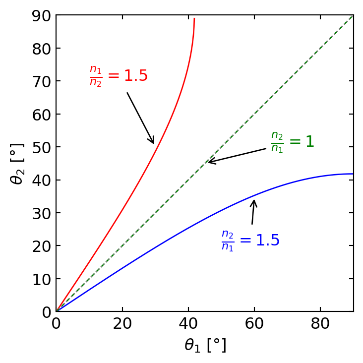
Figure 3— Snell’s law for different combinations of refractive indices. The plots show the relationship between incident angle (\(\theta_1\)) and refracted angle (\(\theta_2\)) for three scenarios: (a) light passing from air to glass, (b) light passing from glass to air, and (c) a comparison of both cases. Note how the curves differ when light moves into a medium with higher refractive index versus a lower refractive index.

Total Internal Reflection

When light travels from a medium with a higher refractive index (\(n_1\)) to one with a lower refractive index (\(n_2\)), a fascinating phenomenon can occur. As the angle of incidence increases, the refracted ray bends away from the normal until, at a critical angle, it travels along the boundary between the two media. Beyond this critical angle, light can no longer pass into the second medium and is instead completely reflected back into the first medium. This phenomenon is known as total internal reflection (TIR).

From Snell’s law, the critical angle \(\theta_c\) occurs when the refracted angle \(\theta_2 = 90°\):

\[n_1\sin\theta_c = n_2\sin(90°) = n_2\]

Therefore:

\[\theta_c = \arcsin\left(\frac{n_2}{n_1}\right)\]

For total internal reflection to occur, two conditions must be satisfied:

Light must travel from a higher to a lower refractive index medium (\(n_1 > n_2\))
The angle of incidence must exceed the critical angle (\(\theta_1 > \theta_c\))

From Fermat’s principle perspective, total internal reflection represents a scenario where no physical path through the second medium can satisfy the minimum optical path length requirement. Instead, the path of least time becomes the reflected path within the original medium. This phenomenon has numerous practical applications, including:

Fiber optic communication: Light signals travel long distances through optical fibers via successive total internal reflections with minimal loss
Prisms and reflectors: Total internal reflection in prisms provides perfect reflection without needing reflective coatings
Gemstones: The brilliance of diamonds results from light being trapped through multiple internal reflections
Optical instruments: Binoculars, periscopes, and endoscopes use prisms with TIR to redirect light

Total internal reflection demonstrates how Fermat’s principle enforces an absolute constraint on light’s behavior—when no path through the second medium can minimize the optical path length, light must remain in the first medium, following the path of least time.

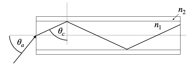
Optical Fibers and Total Internal Reflection

Total internal reflection plays a crucial role in modern telecommunications, particularly in optical fibers, which are also part of many experimental setups. These fibers are essentially ultra-thin glass wires, ranging in diameter from a few micrometers to several hundred micrometers, designed to transport light over long distances with minimal loss.

The structure of an optical fiber is key to its function:

Core: A central glass core with a refractive index \(n_1\)
Cladding: A surrounding layer with a slightly lower refractive index \(n_2\)

This difference in refractive indices is what allows total internal reflection to occur within the fiber.

Figure 4— Total internal reflection in an optical fiber.

For light to propagate effectively through the fiber, it must enter at an angle that ensures total internal reflection at the core-cladding interface. This leads to the concept of the acceptance angle, \(\theta_a\), which is the maximum angle at which light can enter the fiber and still undergo total internal reflection.

To characterize this acceptance angle, optical engineers use a parameter called the Numerical Aperture (NA).

Numerical Aperture

The Numerical Aperture of a fiber is defined as the sine of the maximum acceptance angle:

\[\begin{equation} NA = \sin(\theta_a) = \sqrt{n_1^2 - n_2^2} \end{equation}\]

This equation relates the NA directly to the refractive indices of the core and cladding. The derivation of this formula involves applying Snell’s law at the air-fiber interface and at the core-cladding interface, then using the condition for total internal reflection.

In practice, typical values for the refractive indices might be \(n_1 = 1.475\) for the core and \(n_2 = 1.46\) for the cladding. Plugging these into our equation:

\[\begin{equation} NA = \sqrt{1.475^2 - 1.46^2} \approx 0.2 \end{equation}\]

This means that light entering the fiber within a cone of about 11.5° (arcsin(0.2)) from the fiber’s axis will be transmitted through the fiber via total internal reflection.

The NA is an important parameter in fiber optic design:

It determines the light-gathering ability of the fiber.
It affects the fiber’s bandwidth and its susceptibility to certain types of signal distortion.
It influences how easily the fiber can be coupled to light sources and other fibers.

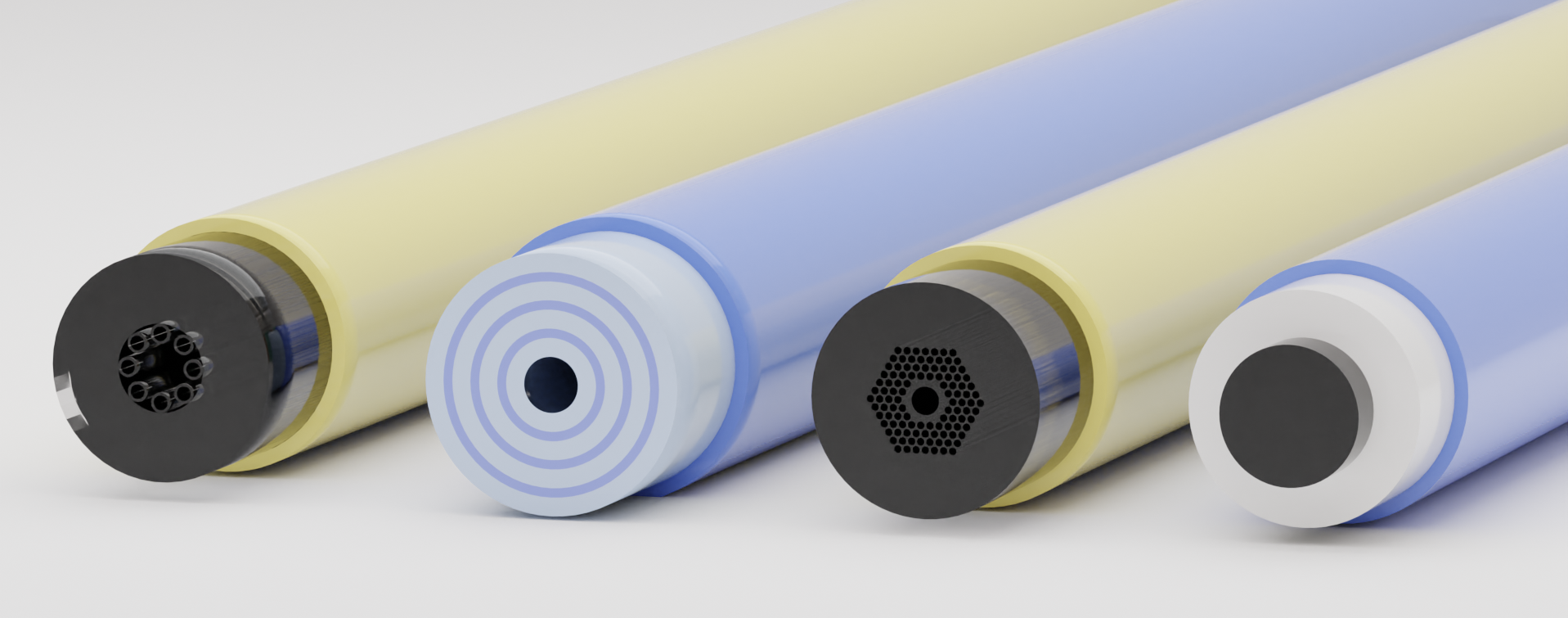
Optical fibers come in various types, each optimized for different applications. Some fibers are designed to transmit light over long distances with minimal loss, while others are engineered for specific wavelengths or to guide light in unusual ways. The figure below shows a few examples of optical fiber types.

Figure 5— Rendering of different optical fibers types (from left to right): Hollow core optical fiber, hollow core bragg fiber, photonic crystal fiber, conventional fiber

Differential Form of Fermat’s Law

To derive the differential ray equation from Fermat’s integral principle, we apply the calculus of variations. Starting with the optical path length functional:

\[L = \int_C n(s)ds = \int_{t_1}^{t_2} n(\mathbf{r}(t)) \left|\frac{d\mathbf{r}}{dt}\right| dt\]

Where \(\mathbf{r}(t)\) parametrizes the path. The term \(\left|\frac{d\mathbf{r}}{dt}\right|\) represents the differential element of arc length \(ds\) along the path, so \(ds = \left|\frac{d\mathbf{r}}{dt}\right| dt\). This parametrization allows us to convert the path integral over the curve \(C\) into a definite integral over the parameter \(t\). According to Fermat’s principle, the true path makes this integral stationary (δL = 0).

Consider a small variation in the path: \(\mathbf{r}(t) \rightarrow \mathbf{r}(t) + \epsilon\mathbf{\eta}(t)\) where \(\mathbf{\eta}(t_1) = \mathbf{\eta}(t_2) = 0\) (fixed endpoints). Expanding the variation of the integral to first order in ε:

\[\delta L = \frac{d}{d\epsilon}\bigg|_{\epsilon=0} \int_{t_1}^{t_2} n(\mathbf{r}(t) + \epsilon\mathbf{\eta}(t)) \left|\frac{d}{dt}(\mathbf{r}(t) + \epsilon\mathbf{\eta}(t))\right| dt\]

Using the chain rule and reparametrizing with arc length \(s\) (where \(\frac{d\mathbf{r}}{ds}\) is a unit vector), the stationarity condition leads to:

\[\int_C \left[ \nabla n \cdot \mathbf{\eta} - \frac{d}{ds}\left(n\frac{d\mathbf{r}}{ds}\right) \cdot \mathbf{\eta} \right] ds = 0\]

Since this must hold for any variation \(\mathbf{\eta}\), we obtain the Euler-Lagrange equation:

\[\frac{d}{ds}\left(n\frac{d\mathbf{r}}{ds}\right) = \nabla n\]

This shows that rays bend toward regions of higher refractive index, directly analogous to how a mechanical particle’s trajectory is affected by a potential field in classical mechanics.

SELFOC Gradient Index Lens

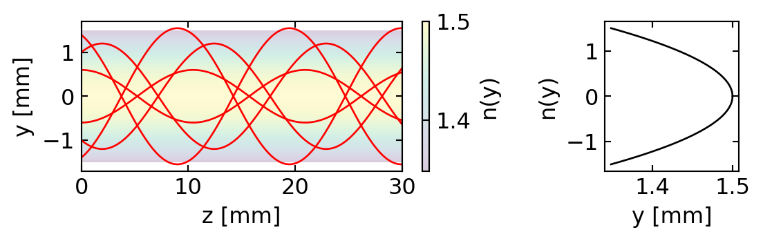
SELFOC (SELf-FOCusing) gradient-index fibers are interesting optical elements that guide light through a continuous refraction process rather than discrete refractions at interfaces. Let me demonstrate how Fermat’s principle can be used to determine the ray paths in these fibers. A SELFOC fiber has a radially varying refractive index, typically following a parabolic profile:

\[n(r) = n_0\left(1 - \frac{1}{2}\alpha^2 r^2\right)\]

where: - \(n_0\) is the refractive index at the central axis - \(r\) is the radial distance from the axis - \(\alpha\) is the gradient constant that determines how quickly the index decreases with radius

Fermat’s Principle in Gradient-Index Media

For a medium with a spatially varying refractive index, Fermat’s principle states that light follows the path that minimizes the optical path length:

\[\delta \int_C n(r) ds = 0\]

This yields the differential equation:

\[\frac{d}{ds}\left(n\frac{d\mathbf{r}}{ds}\right) = \nabla n\]

Deriving the Ray Path Equation

For our parabolic index profile, the gradient of the refractive index is:

\[\nabla n = \frac{\partial n}{\partial r}\hat{\mathbf{r}} = -n_0\alpha^2 r \hat{\mathbf{r}}\]

Using cylindrical coordinates with z along the fiber axis, and assuming the paraxial approximation (rays make small angles with the z-axis), we can simplify the ray equation to:

\[\frac{d^2r}{dz^2} + \alpha^2 r = 0\]

This is the equation for a harmonic oscillator, which has the solution:

\[r(z) = r_0 \cos(\alpha z) + \frac{\theta_0}{\alpha} \sin(\alpha z)\]

where \(r_0\) is the initial radial position and \(\theta_0\) is the initial angle of the ray with respect to the fiber axis.

Code

# Parameters
n0 = 1.5  # Central refractive index
alpha = 0.3  # Gradient constant (mm^-1)
length = 30  # Length of fiber (mm)
radius = 1.5  # Radius of fiber (mm)

# Create a grid for visualization
z = np.linspace(0, length, 300)
r_grid = np.linspace(0, radius, 100)
Z, R = np.meshgrid(z, r_grid)

# Calculate refractive index at each point
N = n0 * (1 - 0.5 * (alpha * R)**2)

# Initialize ray paths
r0_values = [0.6, 1.0, 1.4]  # Initial radial positions
theta0_values = [0, 0.2, -0.2]    # Initial angles (all parallel to axis)

# Plot setup
fig, (ax1, ax2) = plt.subplots(1, 2, figsize=get_size(15, 5), gridspec_kw={'width_ratios': [3, 1]})

# Plot the refractive index profile in the first subplot
cmap = plt.cm.viridis
extent = [0, length, -radius, radius]
im = ax1.imshow(np.vstack((N[::-1], N)), extent=extent,
               aspect='auto', cmap=cmap, origin='lower',alpha=0.2)
fig.colorbar(im, ax=ax1, label='n(y)')

# Plot ray paths
for r0, theta0 in zip(r0_values, theta0_values):
    # Calculate ray path
    r = r0 * np.cos(alpha * z) + (theta0/alpha) * np.sin(alpha * z)

    # Plot ray path
    ax1.plot(z, r, 'r-')
    ax1.plot(z, -r, 'r-')  # Symmetric ray below axis

# Add labels and title for first subplot
ax1.set_xlabel('z [mm]')
ax1.set_ylabel('y [mm]')

# For the right subplot, plot r-position vs refractive index
# Create a finer array of radial positions for a smooth curve
r_positions = np.linspace(0, radius, 100)
# Calculate refractive index at each radial position
n_profile = n0 * (1 - 0.5 * (alpha * r_positions)**2)

# Plot the refractive index profile
ax2.plot( n_profile,r_positions, 'k-')
ax2.plot( n_profile,-r_positions, 'k-')

# Set labels for the index profile subplot
ax2.set_xlabel('y [mm]')
ax2.set_ylabel('n(y)')


plt.tight_layout()
plt.show()

Figure 6— Ray-path inside a SELFOC gradient index optical fiber.

Fermat’s Principle and the “F=ma” Analogy in Optics

The differential form of Fermat’s principle:

\[\frac{d}{ds}\left(n\frac{d\mathbf{r}}{ds}\right) = \nabla n\]

reveals a profound analogy with Newton’s Second Law of motion:

\[\mathbf{F} = m\mathbf{a} = m\frac{d^2\mathbf{r}}{dt^2}\]

This comparison, sometimes called “F=ma optics,” illustrates how light rays follow trajectories mathematically similar to those of mechanical particles. To see this connection more clearly, we can expand the ray equation as:

\[n\frac{d^2\mathbf{r}}{ds^2} + \frac{d\mathbf{r}}{ds}\frac{dn}{ds} = \nabla n\]

Using the chain rule, \(\frac{dn}{ds} = \nabla n \cdot \frac{d\mathbf{r}}{ds}\), and denoting \(\mathbf{t} = \frac{d\mathbf{r}}{ds}\) as the unit tangent vector along the ray:

\[n\frac{d^2\mathbf{r}}{ds^2} + (\nabla n \cdot \mathbf{t})\mathbf{t} = \nabla n\]

Rearranging to isolate the ray curvature term:

\[n\frac{d^2\mathbf{r}}{ds^2} = \nabla n - (\nabla n \cdot \mathbf{t})\mathbf{t}\]

The right side represents the component of \(\nabla n\) perpendicular to the ray direction, which we can denote as \((\nabla n)_\perp\). Therefore:

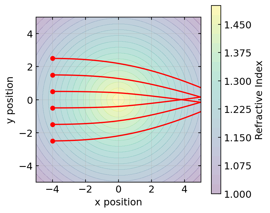
\[\frac{d^2\mathbf{r}}{ds^2} = \frac{1}{n}(\nabla n)_\perp\]

This equation reveals that the ray curvature is proportional to the perpendicular component of the refractive index gradient and inversely proportional to the refractive index itself. Crucially, this shows that light rays bend toward regions of higher refractive index, not away from them.

This behavior explains many optical phenomena:

Light bending toward the normal when entering a medium with higher refractive index
Light guiding in optical fibers where light remains confined in the higher-index core
Formation of mirages where light curves toward the denser air near the ground
Focusing in gradient-index (GRIN) lenses where the refractive index decreases radially from the center

While the mathematical form resembles Newton’s equation for particle motion, the analogy must be carefully interpreted: unlike particles that accelerate toward lower potential energy, light rays curve toward regions of higher refractive index.

Code

# Parameters
n0 = 1.5  # Base refractive index (center value)
n_min = 1.0  # Minimum refractive index (at edges)
x_range = np.linspace(-5, 5, 100)
y_range = np.linspace(-5, 5, 100)
X, Y = np.meshgrid(x_range, y_range)

# Calculate radial distance from center
R = np.sqrt(X**2 + Y**2)
# Max radius in our plot
R_max = 5*np.sqrt(2)

# Create a refractive index profile that decreases with radius
# but never goes below n_min
gradient_strength = (n0 - n_min)/R_max  # Calculate appropriate gradient strength
n = n0 - gradient_strength * R  # Linear decrease with radius

# Set up the figure
fig, ax = plt.subplots(figsize=get_size(12, 10))

# Plot the refractive index as a contour plot
contour = ax.contourf(X, Y, n, 20, cmap='viridis', alpha=0.3)
cbar = fig.colorbar(contour, ax=ax, label='Refractive Index')

# Calculate and plot some ray trajectories
# We'll simulate the paths by numerical integration

def ray_path(r0, v0, steps=1000, dt=0.05):
    """Simulate a ray path through the medium"""
    r = np.zeros((steps, 2))
    v = np.zeros((steps, 2))
    r[0] = r0
    v[0] = v0 / np.linalg.norm(v0)  # Normalize velocity

    for i in range(1, steps):
        # Get position
        x, y = r[i-1]
        if abs(x) >= 5 or abs(y) >= 5:
            return r[:i]

        # Approximate gradient of n at this point
        eps = 0.01
        nx_plus = n0 - gradient_strength * np.sqrt((x+eps)**2 + y**2)
        nx_minus = n0 - gradient_strength * np.sqrt((x-eps)**2 + y**2)
        ny_plus = n0 - gradient_strength * np.sqrt(x**2 + (y+eps)**2)
        ny_minus = n0 - gradient_strength * np.sqrt(x**2 + (y-eps)**2)

        grad_n_x = (nx_plus - nx_minus) / (2*eps)
        grad_n_y = (ny_plus - ny_minus) / (2*eps)
        grad_n = np.array([grad_n_x, grad_n_y])

        # Current n value
        current_n = n0 - gradient_strength * np.sqrt(x**2 + y**2)

        # Calculate the perpendicular component of gradient
        t = v[i-1] / np.linalg.norm(v[i-1])  # Tangent vector (normalized velocity)
        grad_n_parallel = np.dot(grad_n, t) * t  # Component along ray direction
        grad_n_perp = grad_n - grad_n_parallel  # Perpendicular component

        # Update velocity - rays bend toward higher refractive index
        a = grad_n_perp / current_n
        v[i] = v[i-1] + a * dt
        v[i] = v[i] / np.linalg.norm(v[i])  # Ensure unit speed

        # Update position
        r[i] = r[i-1] + v[i] * dt

    return r

# Calculate several ray paths
start_positions = [
    [-4, 2.5], [-4, 1.5], [-4, 0.5],
    [-4, -0.5], [-4, -1.5], [-4, -2.5]
]
paths = []

for start_pos in start_positions:
    path = ray_path(start_pos, [1, 0], steps=500)
    paths.append(path)
    ax.plot(path[:, 0], path[:, 1], 'r-', linewidth=1.5)

# Add start points
for pos in start_positions:
    ax.plot(pos[0], pos[1], 'ro')

# Add axis labels
ax.set_xlabel('x position')
ax.set_ylabel('y position')
ax.set_xlim(-5, 5)
ax.set_ylim(-5, 5)
ax.set_aspect('equal')
ax.grid(True, alpha=0.3)

plt.tight_layout()
plt.show()

Figure 7— F=ma optics - Light rays (red) following paths toward regions of higher refractive index

Lenses

Lenses are among the most fundamental optical elements in photonics, using curved surfaces (typically spherical) to manipulate light paths. Understanding how lenses work requires analyzing refraction at spherical surfaces and applying this to the thin lens model.

Refraction at Spherical Surfaces

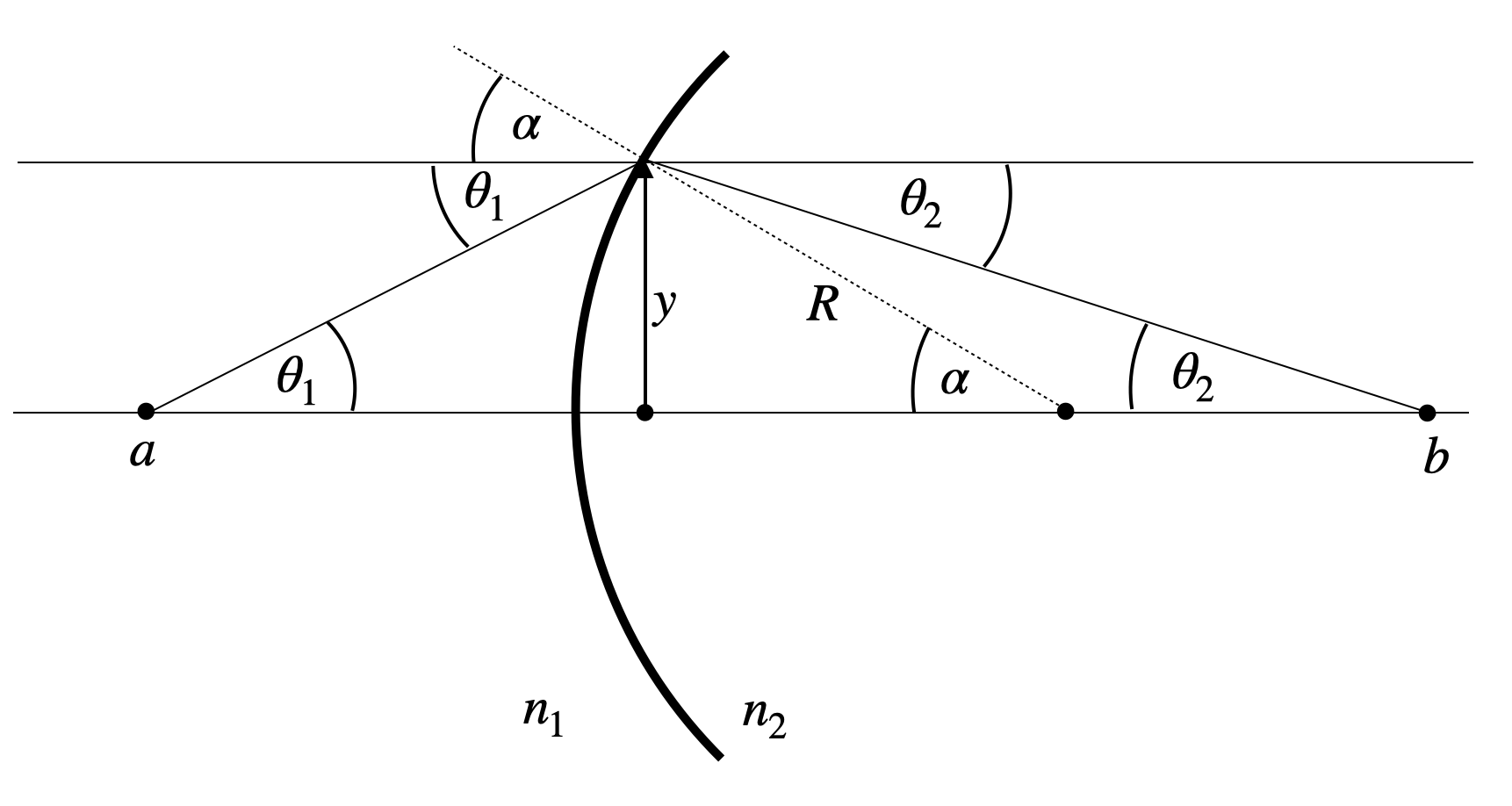
When light encounters a spherical boundary between two media, we can analyze its path using Snell’s law and geometric considerations as shown below:

Figure 8— Refraction at a curved surface.

To determine how an image forms, we need to find where rays originating from a point at distance \(a\) from the surface will converge after refraction. Using Snell’s law for a ray hitting the surface at angle \(\alpha+\theta_1\):

\[n_{1}\sin(\alpha+\theta_1)=n_{2}\sin(\alpha-\theta_2)\]

Where: \[\sin(\alpha)=\frac{y}{R}, \quad \tan(\theta_1)=\frac{y}{a}, \quad \tan(\theta_2)=\frac{y}{b}\]

For practical optical systems, we employ the paraxial approximation, where all angles are assumed small enough that:

\[\sin(\theta) \approx \theta+ O(\theta^{3}), \quad \tan(\theta) \approx \theta + O(\theta^{3}),\quad \cos(\theta)\approx 1 + O(\theta^{2})\]

This simplifies Snell’s law to:

\[n_1(\alpha+\theta_1)=n_2(\alpha-\theta_2)\]

After appropriate transformations (detailed in the online lecture), we obtain:

\[\theta_2=\frac{n_2-n_1}{n_2 R}y -\frac{n_1}{n_2}\theta_1\]

This linear relationship between input (\(y\), \(\theta_1\)) and output (\(\theta_2\)) parameters is a hallmark of paraxial optics.

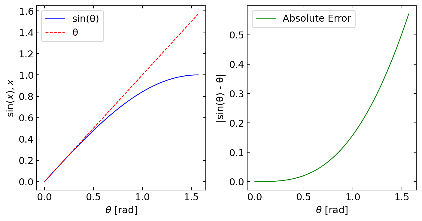
Paraxial Approximation

The paraxial approximation is a fundamental simplification in optics that assumes all angles are small. This allows us to use linear approximations for trigonometric functions, significantly simplifying calculations while maintaining accuracy for most practical scenarios involving lenses.

To visualize the validity of this approximation, let’s examine two plots:

The first plot compares sin(θ) (blue line) with its linear approximation θ (red dashed line) for angles ranging from 0 to π/2 radians.
The second plot shows the absolute error between sin(θ) and θ.

These plots demonstrate that:

For small angles (roughly up to 0.5 radians or about 30 degrees), the approximation is very close to the actual sine function.
The error increases rapidly for larger angles, indicating the limitations of the paraxial approximation.

In most optical systems, especially those involving lenses, the angles of incident and refracted rays are typically small enough for this approximation to be valid. However, it’s important to be aware of its limitations when dealing with wide-angle optical systems or scenarios where precision is critical.

Code

import numpy as np
import matplotlib.pyplot as plt
# Define the range of angles (in radians)
theta = np.linspace(0, np.pi/2, 1000)

# Calculate sin(theta) and theta (linear approximation)
sin_theta = np.sin(theta)
linear_approx = theta

# Calculate the absolute error
error = np.abs(sin_theta - linear_approx)

# Create the plot with two subplots side by side
fig, (ax1, ax2) = plt.subplots(1, 2, figsize=(7.5, 4))

# Plot sin(theta) and theta on the first subplot
ax1.plot(theta, sin_theta, label='sin(θ)', color='blue')
ax1.plot(theta, linear_approx, label='θ', color='red', linestyle='--')
ax1.set_xlabel(r'$\theta$ [rad]')
ax1.set_ylabel(r'$\sin(x),x$')
ax1.legend()

# Plot the error on the second subplot
ax2.plot(theta, error, label='Absolute Error', color='green')
ax2.set_xlabel(r'$\theta$ [rad]')
ax2.set_ylabel('|sin(θ) - θ|')
ax2.legend()

# Adjust the layout and display the plot
plt.tight_layout()
plt.show()

Visualization of the paraxial approximation plotting the \(\sin(\theta)\) and the linear approximation \(\theta\) (dashed line) for angles ranging from 0 to \(\pi/2\) radians.

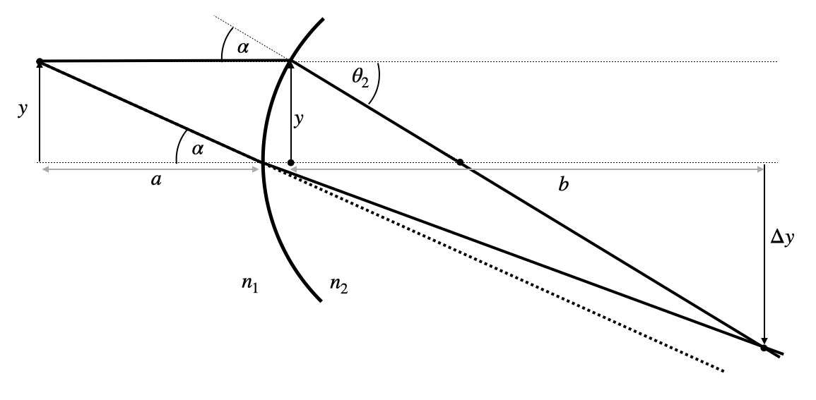
To derive the imaging equation, we analyze how light from a point object forms an image after refraction. Consider two special rays from an off-axis point:

Figure 9— Image formation at a curved surface.

For a ray parallel to the optical axis (\(\theta_1=0\)):

\[\theta_2=\frac{n_2-n_1}{n_2}\frac{y}{R}=\frac{y+\Delta y}{b}\]

For a ray through the center of curvature (\(y=0\)):

\[n_2\frac{\Delta y}{b}=n_1\frac{y}{a}\]

Combining these equations yields the fundamental imaging equation for a spherical surface:

\[\frac{n_1}{a}+\frac{n_2}{b}=\frac{n_2-n_1}{R}\]

From this, we define the focal length of the spherical surface:

\[f=\frac{n_2}{n_2-n_1}R\]

Imaging Equation for Spherical Refracting Surface

The sum of the inverse object and image distances equals the inverse focal length of the spherical refracting surface:

\[\frac{n_1}{a}+\frac{n_2}{b}\approx\frac{n_2}{f}\]

where the focal length of the refracting surface is given by:

\[f=\frac{n_2}{n_2-n_1}R\]

in the paraxial approximation.

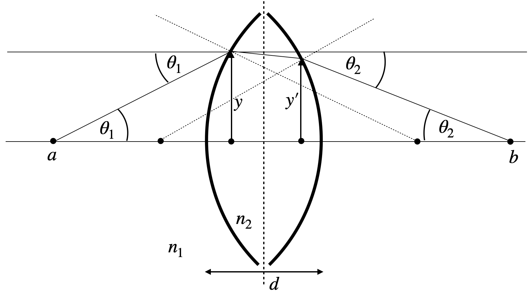
Thin Lens

A lens consists of two spherical surfaces in close proximity. To analyze how a lens forms images, we consider refraction at both surfaces:

Figure 10— Refraction on two spherical surfaces.

When the lens thickness \(d\) is much smaller than the radii of curvature (\(d \ll R_1, R_2\)), we can apply the thin lens approximation. This assumes: 1. The ray height at both surfaces is approximately equal (\(y \approx y'\)) 2. All refraction effectively occurs at a single plane (the principal plane) 3. The change in angle is additive from both surfaces

This approximation, combined with the sign convention for radii (positive for convex surfaces facing incoming light, negative for concave), leads to the thin lens formula:

Imaging Equation for Thin Lens

The sum of the inverse object and image distances equals the inverse focal length of the thin lens:

\[\frac{1}{a}+\frac{1}{b}=\frac{1}{f}\]

where:

\[\frac{1}{f}=\frac{n_2-n_1}{n_1}\left(\frac{1}{R_1}-\frac{1}{R_2}\right)\]

This can be rearranged to give the lensmaker equation:

Lensmaker Equation

The focal length of a thin lens is calculated by: \[f=\frac{n_1}{n_2-n_1}\left(\frac{R_1 R_2}{R_2-R_1}\right)\]

in the paraxial approximation.

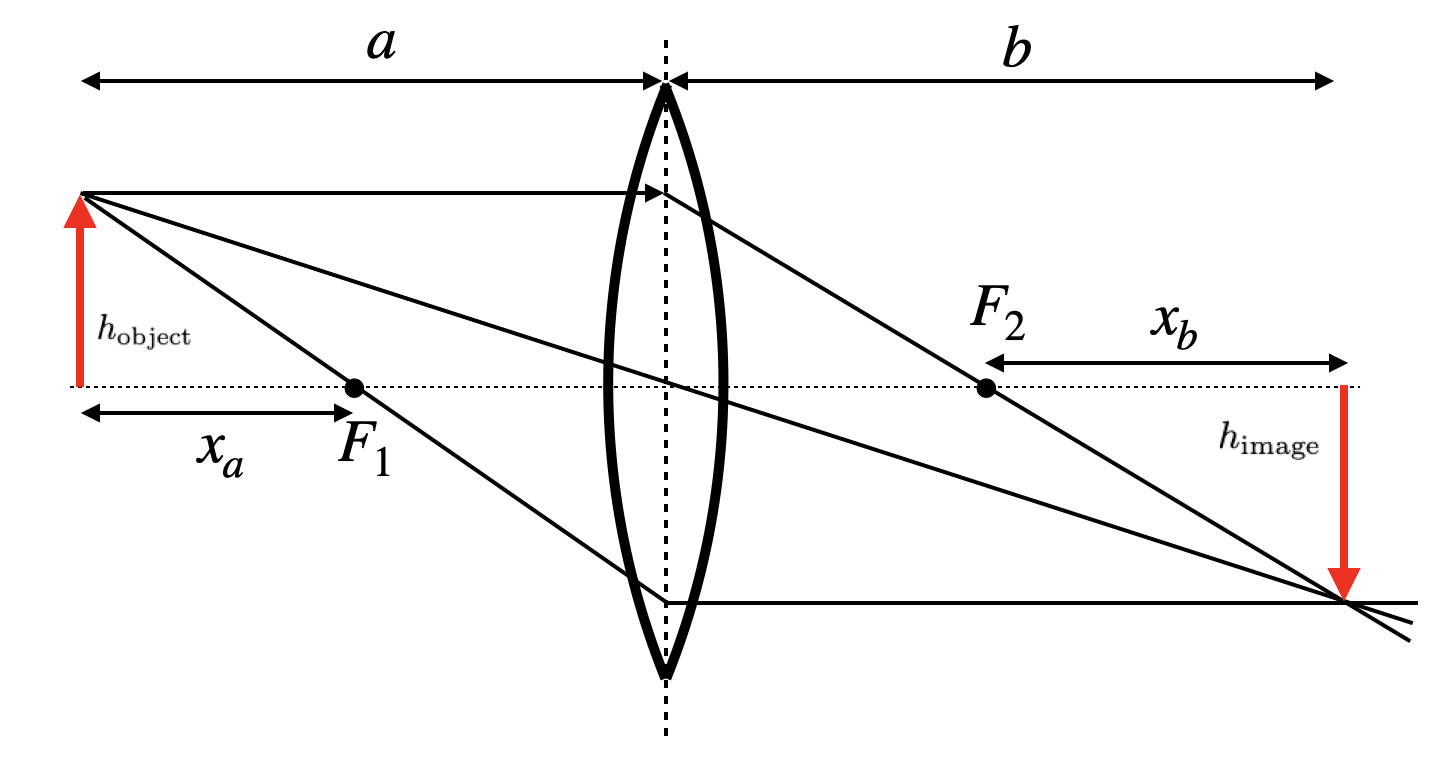
Image Construction and Magnification

To construct the image formed by a lens, we typically trace two or three special rays: 1. A ray parallel to the optical axis, which passes through the far focal point after refraction 2. A ray through the center of the lens, which passes undeflected 3. A ray through the near focal point, which emerges parallel to the optical axis

The intersection of these rays locates the image position:

Figure 11— Image construction on a thin lens.

The ratio of image height to object height defines the magnification:

Magnification of a Lens

The magnification is given by:

\[M=\frac{h_{\rm image}}{h_{\rm object}}=-\frac{b}{a}=\frac{f}{f-a}\]

where the negative sign indicates image inversion for real images.

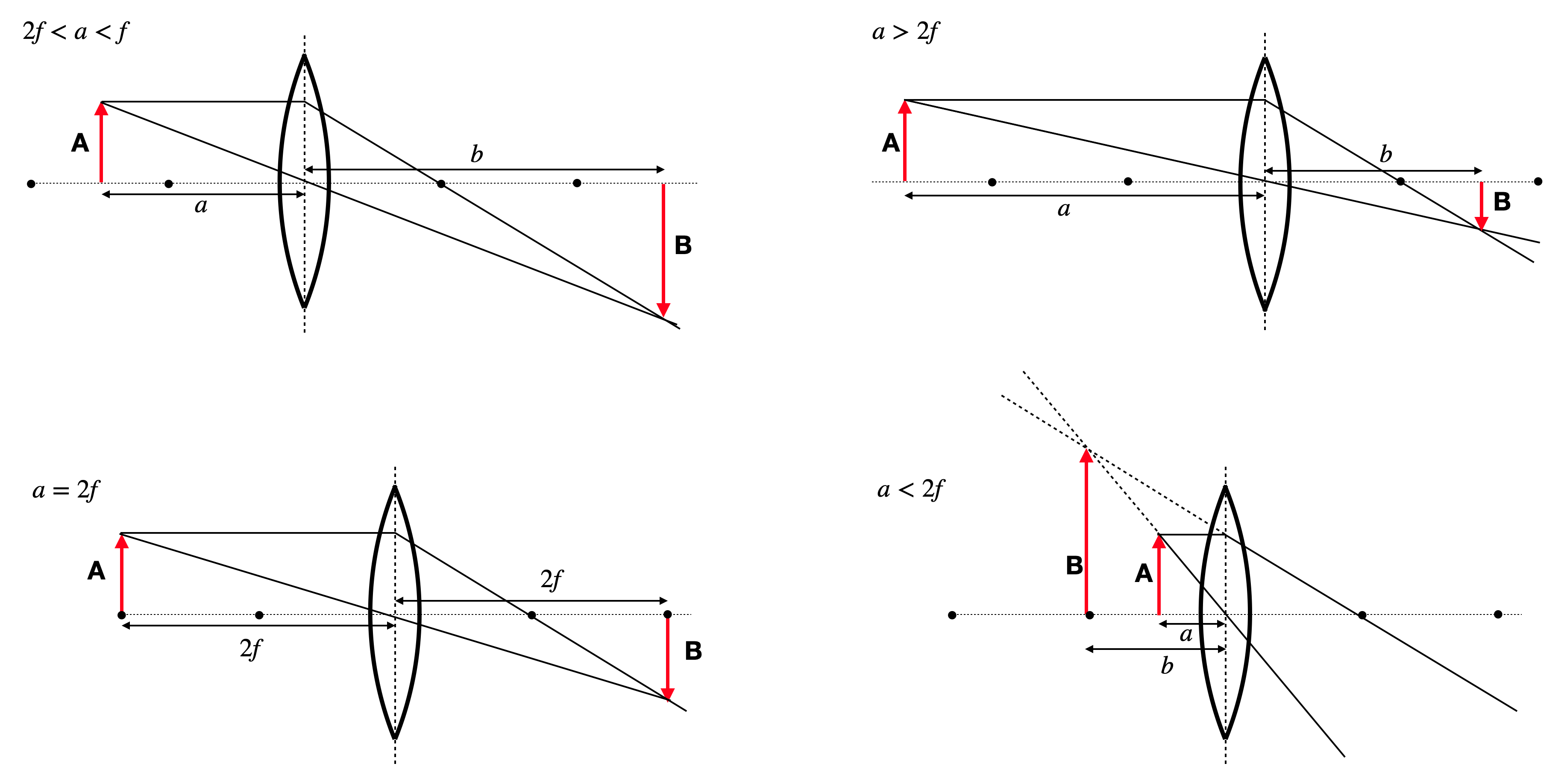
The image characteristics depend on the object distance relative to the focal length:

Object Position	Image Characteristics	Magnification (M)	Image Type
\(a < f\)	Upright and magnified	\(M > 0\)	Virtual
\(f < a < 2f\)	Inverted and magnified	\(M < -1\)	Real
\(a = 2f\)	Inverted, same size	\(M = -1\)	Real
\(a > 2f\)	Inverted and reduced	\(-1 < M < 0\)	Real
\(a = f\)	Image at infinity	\(M = \infty\)	-

The diagram below illustrates these various imaging scenarios for a biconvex lens:


Fig.: Image construction on a biconvex lens with a parallel and a central ray for different object distances.

Matrix Optics

The above derived equations for a single spherical surface yield a linear relation between the input variables \(y_1\) and \(\theta_1\) and the output variables \(y_2\) and \(\theta_2\). The linear relation yields a great opportunity to express optical elements in terms of linear transformations (matrices). This is the basis of matrix optics. The matrix representation of a lens is given by

\[\begin{pmatrix} y_2 \\ \theta_2 \end{pmatrix} = \begin{pmatrix} 1 & 0 \\ -\frac{1}{f} & 1 \end{pmatrix} \begin{pmatrix} y_1 \\ \theta_1 \end{pmatrix}\]

where the matrix is called the ABCD matrix of the lens. Due to the linearization of Snells law w can write down more generally

\[\begin{pmatrix} y_2 \\ \theta_2 \end{pmatrix} = \begin{pmatrix} A & B \\ C & D \end{pmatrix} \begin{pmatrix} y_1 \\ \theta_1 \end{pmatrix}\]

and one can obtain a Matrix for all types of optical elements such as free space of dustance \(d\).

\[\begin{bmatrix} A & B\\ C & D \end{bmatrix} = \begin{bmatrix} 1 & d\\ 0 & 1 \end{bmatrix} \]

Here are some useful matrices for optical elements:

\[ \mathbf{M}=\left[\begin{array}{ll} 1 & d \\ 0 & 1 \end{array}\right] \tag{Free space} \]

\[ \mathbf{M}=\left[\begin{array}{cc} 1 & 0 \\ 0 & \frac{n_1}{n_2} \end{array}\right] \tag{Planar interface} \]

\[ \mathbf{M}=\left[\begin{array}{cc} 1 & 0 \\ -\frac{\left(n_2-n_1\right)}{n_2 R} & \frac{n_1}{n_2} \end{array}\right] \tag{Spherical Boundary} \]

\[ \mathbf{M}=\left[\begin{array}{cc} 1 & 0 \\ -\frac{1}{f} & 1 \end{array}\right] \tag{Tin Lens} \]

If we have now a system of optical elements, we can multiply the matrices of the individual elements to obtain the matrix of the whole system.

\[ \rightarrow \mathrm{M}_1 \rightarrow \mathrm{M}_2 \rightarrow \mathrm{M}_N \rightarrow \mathrm{M}=\mathbf{M}_N \ldots \mathrm{M}_2 \mathbf{M}_1 \text {. } \]

This is a very powerful tool to analyze optical systems.

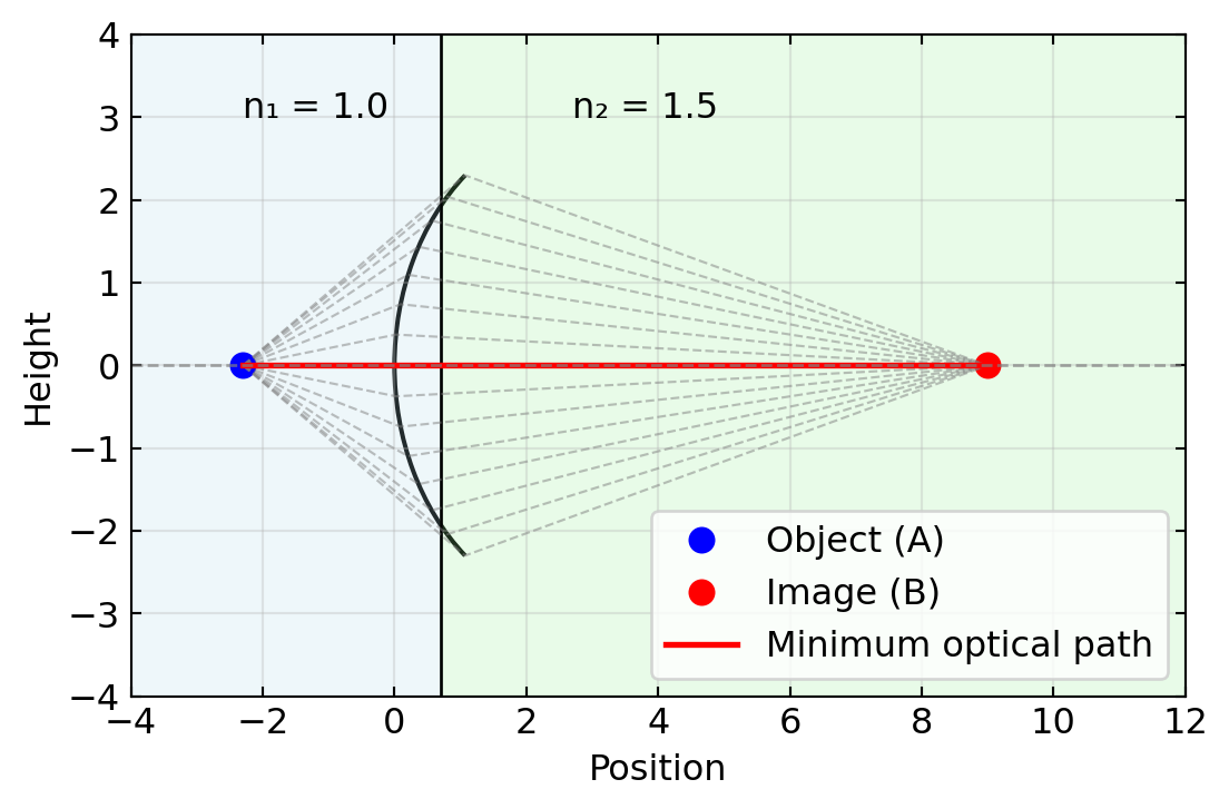
Fermat’s Principle for Spherical Surfaces

The power of Fermat’s principle becomes particularly evident when applied to spherical refracting surfaces. Consider a spherical boundary of radius \(R\) between two media with refractive indices \(n_1\) and \(n_2\). According to Fermat’s principle, light will follow the path that minimizes the total optical path length.

Code

import numpy as np
import matplotlib.pyplot as plt
from matplotlib.patches import Arc, Wedge
import matplotlib.patches as patches

# Set up the figure
fig, ax = plt.subplots(figsize=get_size(15, 10))

# Parameters
R = 3  # Radius of the spherical surface
n1 = 1.0  # Refractive index of first medium
n2 = 1.5  # Refractive index of second medium
arc_angle = 100  # Arc angle in degrees
center_x = 3  # Center of arc is to the right of the boundary

# Define the center of the sphere
center = (center_x, 0)

# Calculate arc angles in radians
start_angle = 180 - arc_angle/2
end_angle = 180 + arc_angle/2

# Draw the spherical surface as an arc
arc = Arc(center, 2*R, 2*R, theta1=start_angle, theta2=end_angle,
          color='black', linewidth=1.5)
ax.add_patch(arc)

# Calculate the x-coordinate of the leftmost point of the arc
boundary_x = center_x - R * np.cos(np.radians(90 - arc_angle/2))

# Draw the media boundary
ax.fill_between([-8, boundary_x], [-8, -8], [8, 8], color='lightblue', alpha=0.2)
ax.fill_between([boundary_x, 12], [-8, -8], [8, 8], color='lightgreen', alpha=0.2)
ax.axvline(x=boundary_x, color='black', linestyle='-', linewidth=1)

# Add labels for the media
ax.text(boundary_x-3, 3, f"n₁ = {n1}", fontsize=12)
ax.text(boundary_x+2, 3, f"n₂ = {n2}", fontsize=12)

# Mark object and image points
object_point = (boundary_x-3, 0)
image_point = (center_x+6, 0)
ax.plot(object_point[0], object_point[1], 'bo', markersize=8, label='Object (A)')
ax.plot(image_point[0], image_point[1], 'ro', markersize=8, label='Image (B)')

# Calculate different potential paths along the arc
theta_rad = np.linspace(np.radians(start_angle), np.radians(end_angle), 15)
paths = []
optical_lengths = []

for theta in theta_rad:
    # Position on the arc
    x = center_x + R * np.cos(theta)
    y = R * np.sin(theta)

    # Calculate distances
    d1 = np.sqrt((x - object_point[0])**2 + (y - object_point[1])**2)
    d2 = np.sqrt((x - image_point[0])**2 + (y - image_point[1])**2)

    # Calculate optical path length
    optical_length = n1 * d1 + n2 * d2

    paths.append((x, y))
    optical_lengths.append(optical_length)

# Find the minimum optical path
min_index = np.argmin(optical_lengths)
min_path = paths[min_index]

# Plot all potential paths
for i, (x, y) in enumerate(paths):
    if i == min_index:
        continue
    ax.plot([object_point[0], x, image_point[0]], [object_point[1], y, image_point[1]],
             'gray', linestyle='--', alpha=0.5, linewidth=0.8)

# Plot the path of minimum optical length (Fermat's principle)
ax.plot([object_point[0], min_path[0], image_point[0]], [object_point[1], min_path[1], image_point[1]],
         'red', linewidth=2, label='Minimum optical path')


# Set up the main plot
ax.set_xlim(-4, 12)
ax.set_ylim(-4, 4)
ax.set_xlabel('Position')
ax.set_ylabel('Height')
ax.grid(True, alpha=0.3)
ax.axhline(y=0, color='gray', linestyle='--', alpha=0.7)
ax.legend(loc='lower right')

plt.tight_layout()
plt.show()

Figure 12— Fermat’s principle applied to a spherical refracting surface

When we apply Fermat’s principle to a spherical surface, we can derive the laws of refraction. Consider a spherical boundary between two media with refractive indices \(n_1\) and \(n_2\). We’ll place our coordinate system so that the spherical surface intersects the x-axis at x=0, with radius R and its center at position (R,0) to the right.

For a point P on the spherical surface at height y from the optical axis, the total optical path length from object point A at (-a,0) to image point B at (b,0) is:

\[L = n_1|AP| + n_2|PB|\]

where: \[|AP| = \sqrt{a^2 + y^2}\] \[|PB| = \sqrt{b^2 + y^2}\]

According to Fermat’s principle, light follows the path where this length is stationary:

\[\frac{dL}{dy} = n_1\frac{d|AP|}{dy} + n_2\frac{d|PB|}{dy} = 0\]

Computing these derivatives:

\[\frac{d|AP|}{dy} = \frac{y}{|AP|}\] \[\frac{d|PB|}{dy} = \frac{y}{|PB|}\]

Substituting into our condition:

\[n_1\frac{y}{|AP|} + n_2\frac{y}{|PB|} = 0\]

This equation is incorrect. The right-hand side should not be zero because we need to account for the geometry of the spherical surface. The correct form includes the effect of the surface normal:

\[n_1\frac{y}{|AP|} + n_2\frac{y}{|PB|} = \frac{(n_2-n_1)y}{R}\]

This correction comes from the fact that at point P, the normal to the spherical surface makes an angle α with the optical axis, where sin(α) ≈ y/R in the paraxial approximation.

Dividing by y (assuming y≠0):

\[\frac{n_1}{|AP|} + \frac{n_2}{|PB|} = \frac{n_2-n_1}{R}\]

In the paraxial approximation, we can use |AP| ≈ a and |PB| ≈ b, yielding:

\[\frac{n_1}{a} + \frac{n_2}{b} = \frac{n_2-n_1}{R}\]

This is the correct imaging equation for a spherical refracting surface.

The elegance of Fermat’s principle is preserved, as it still naturally produces the same result as our geometric derivation, once we properly account for the geometry of the refracting surface.

Deriving the Thin Lens Equation from Fermat’s Principle

To derive the thin lens equation, we apply Fermat’s principle to the two spherical surfaces that make up a lens. Consider a lens with refractive index \(n_2\) in a medium of index \(n_1\), with surface radii \(R_1\) and \(R_2\).

The total optical path for a ray passing through the lens at height \(y\) from the optical axis is: - Path from object to first surface: \(n_1 s_1\) - Path through the lens: \(n_2 s_2\) - Path from second surface to image: \(n_1 s_3\)

For a thin lens, the optical path length simplifies to:

\[L(y) = n_1 \sqrt{a^2 + y^2} + n_2 d(y) + n_1 \sqrt{b^2 + y^2}\]

Where \(d(y)\) is the thickness of the lens at height \(y\), which can be approximated as:

\[d(y) \approx d_0 + \frac{y^2}{2}\left(\frac{1}{R_1}-\frac{1}{R_2}\right)\]

Applying Fermat’s principle (\(\frac{dL}{dy} = 0\)) and using the paraxial approximation:

\[\frac{n_1 y}{\sqrt{a^2 + y^2}} + n_2 y \left(\frac{1}{R_1}-\frac{1}{R_2}\right) + \frac{n_1 y}{\sqrt{b^2 + y^2}} = 0\]

In the paraxial limit (\(y \ll a, y \ll b\)), this becomes:

\[\frac{n_1 y}{a} + n_2 y \left(\frac{1}{R_1}-\frac{1}{R_2}\right) + \frac{n_1 y}{b} = 0\]

Dividing by \(y\) and rearranging:

\[\frac{1}{a} + \frac{1}{b} = \frac{n_2-n_1}{n_1}\left(\frac{1}{R_1}-\frac{1}{R_2}\right) = \frac{1}{f}\]

This is the thin lens equation with the focal length given by the lensmaker’s equation:

\[f = \frac{n_1}{n_2-n_1}\left(\frac{R_1 R_2}{R_2-R_1}\right)\]

Thus, both the imaging equation and the lensmaker equation emerge naturally from Fermat’s principle applied to the geometry of a thin lens, showing that light follows paths of equal optical length from object to image when passing through any part of the lens.

From a wave perspective, what makes a lens focus light to a point is that all paths from object to image through any part of the lens have equal optical path lengths (to first order in the paraxial approximation), ensuring constructive interference at the image point.