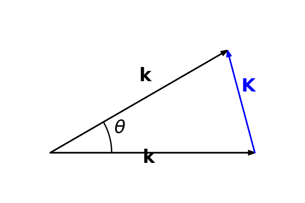
The QLSI result is a special case of a much more general idea: an extra phase profile \(\phi(x)\) imposed within each period of a periodic structure controls how the energy is distributed among the diffraction orders, while the period \(d\) alone fixes their angular positions through \(d\sin\theta_m = m\lambda\).
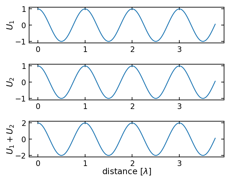
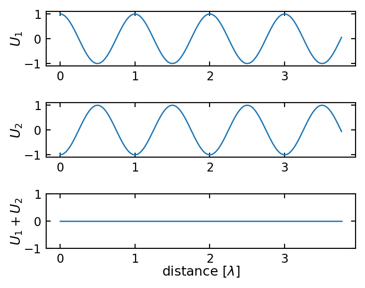
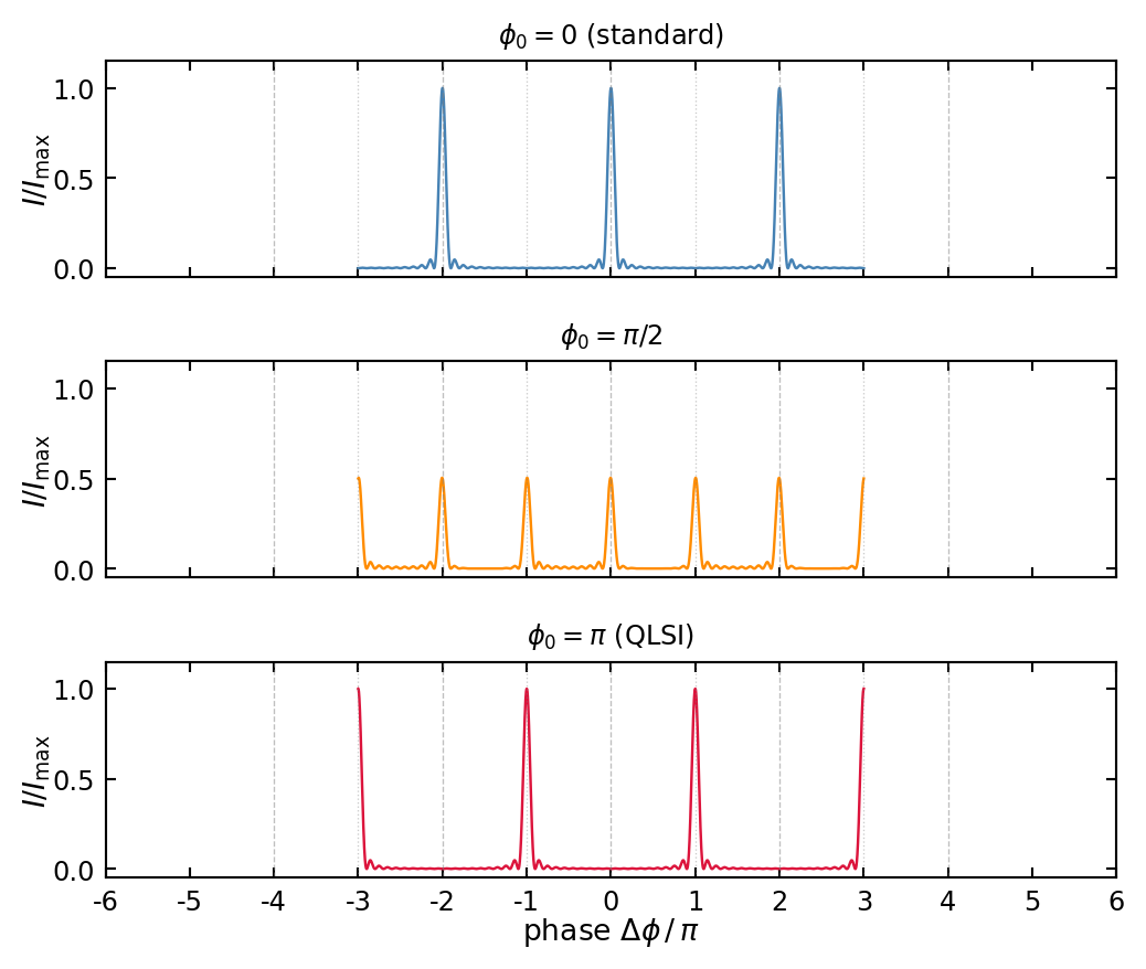
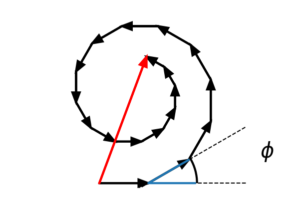
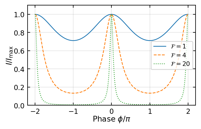
In Eq. 3 the multi-slit factor \(\sin^2(N\Delta\phi)/\sin^2(\Delta\phi)\) sets the positions of the principal maxima, and the prefactor \(4\cos^2((\Delta\phi+\phi_0)/2)\) — the Fourier transform of the two-element phase pattern \(\{1, e^{i\phi_0}\}\) — sets their relative weights. Choosing \(\phi_0=\pi\) zeroes the even orders (QLSI). Choosing a different \(\phi(x)\) within a period redistributes the weights differently.
Blazed gratings. A blazed grating takes this idea to its extreme: instead of a binary \(0/\pi\) step, it imposes a linear phase ramp
\[
\phi(x) = \frac{2\pi}{d}\,x \sin\theta_B,\qquad 0\le x<d,
\]
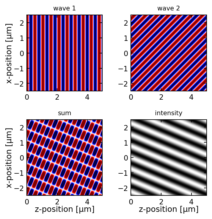
within each period, repeating sawtooth-like from period to period. This is exactly the phase profile of a plane wave tilted by the blaze angle \(\theta_B\). Its per-period Fourier transform is concentrated on a single diffraction order — the one whose angle matches \(\theta_B\) — so essentially all the diffracted energy is steered into that order, while all others (including the 0th) are suppressed. Physically the linear phase ramp is realised by tilting the reflecting (or transmitting) facets of each groove by \(\theta_B\), so that specular reflection from the facet and diffraction from the grating point in the same direction.
Acousto-optic modulators (AOMs). The phase profile does not have to be etched into the substrate — it can also be written dynamically by sound. In an AOM, an RF transducer launches an ultrasonic wave at frequency \(\Omega\) into a transparent crystal (TeO₂, fused silica, PbMoO₄…). Through the photoelastic effect, the strain modulates the refractive index as
\[
\Delta n(x,t) = \Delta n_0 \cos(Kx-\Omega t),\qquad K = \frac{2\pi}{\Lambda} = \frac{\Omega}{v_s},
\]
where \(\Lambda\) is the acoustic wavelength and \(v_s\) the speed of sound. A light beam traversing an interaction length \(L\) picks up a sinusoidal phase grating
\[
\phi(x,t) = k_0\,\Delta n_0\, L\,\cos(Kx-\Omega t),
\]
which is exactly the same kind of per-period phase modulation as in QLSI or a blazed grating — only now the profile is sinusoidal, dynamic, and moving. The Fourier coefficients of \(e^{i\phi_0\cos\theta}\) are Bessel functions \(J_m(\phi_0)\), so the diffracted orders carry intensities \(\propto J_m^2(\phi_0)\) and their weights are tunable in real time via the RF drive amplitude.
Two features are unique to the acousto-optic case:
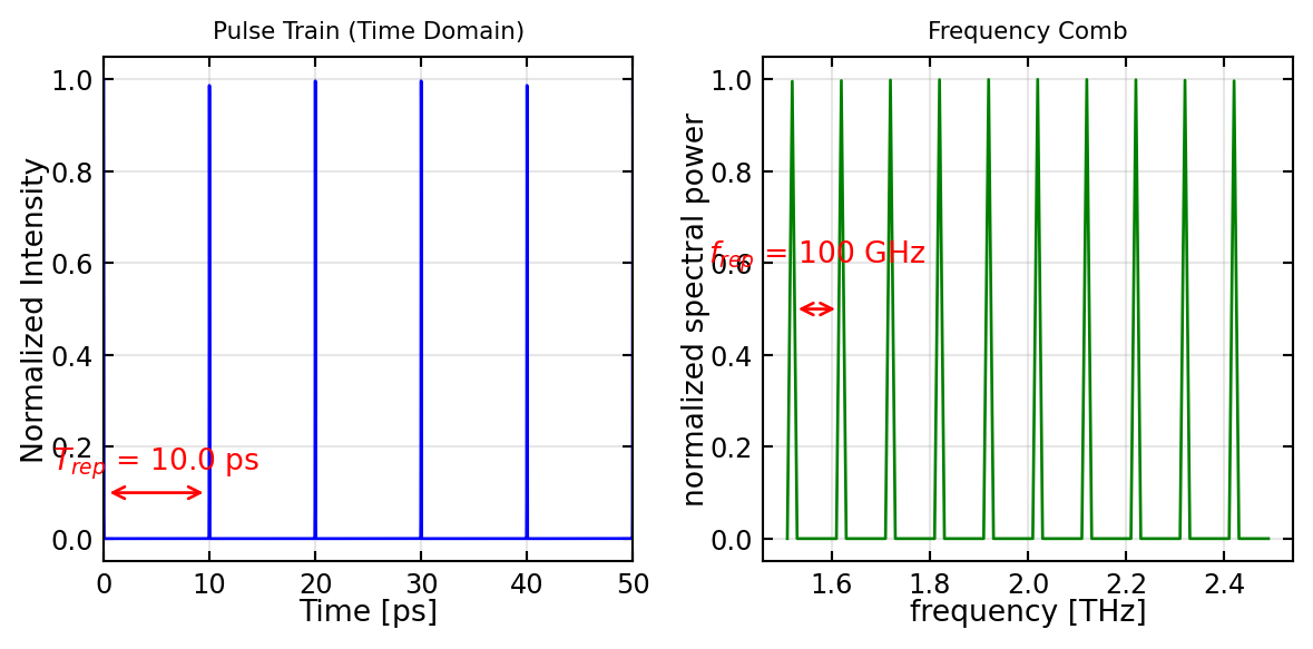
- Tunable deflection angle. Because \(\Lambda = v_s/\Omega\), changing the RF frequency \(\Omega\) rescales the grating period and hence the diffraction angle \(\sin\theta_m = m\lambda/\Lambda\). AOMs are therefore widely used as fast, electronically steered beam deflectors, optical switches, and pulse pickers.
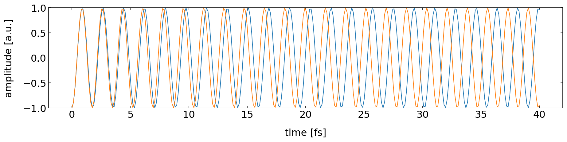
- Doppler shift. Because the grating moves with the sound wave, photon–phonon energy conservation shifts the \(m\)-th order in frequency by \(m\Omega\): the diffracted light is frequency-shifted by the RF drive, which is the basis of laser frequency stabilisation, heterodyne detection, and laser cooling of atoms.
In the thick-grating (Bragg) regime only a single order survives — just as for a blazed grating — typically with \(>80\%\) diffraction efficiency.
The full hierarchy now reads:
| Constant (\(\phi_0=0\)) |
Plain amplitude grating |
0th order strongest, symmetric pattern |
| Two-step \(0,\pi\) |
Etched \(\pi\)-checkerboard |
Even orders suppressed (QLSI) |
| Linear ramp |
Tilted groove facets |
All energy into one order (blazed grating) |
| Sinusoidal, travelling |
Acoustic wave in a crystal |
Tunable, frequency-shifting AOM |
In each case, an engineered sub-period phase profile decides where — and at what frequency — the diffracted light goes.