33 Semidilute Polymer Solutions
The properties of polymer solutions change when you increase the density of the solution. In the case of dilite solutions, we have already seen that the viscosity changes linearly with the concentration of the polymer. Whe the chains start to overlap, the neigboring chains impose constraints which influence the relaxation of the chains upon deformation.
To identify, when such a semi-dilute regime is reached, we can have a look at the volume fraction
\[ \phi=\frac{n V b^{3}}{V} \]
where \(n\) is the number of polymer chains, \(V\) is the sample vlume and \(N\) is the number of Kuhn segements of length \(b\). If we have now polymer chains of a size \(R\) (end-to-end distance), with a volume of \(R^3\) we can then fill our sample volume space filling with \(n\) chains such that the sample volume \(V=nR^3\). This results in a concentration that is given by
\[ \phi^{*}\approx \frac{Nb^3}{R^3} \]
which is the overlap concentration indicating that the chains start to overlap at this concentration. Since the size \(R\) of the chain can be now expressed by
\[ R\approx b \left (\frac{v}{b^{3}}\right )^{2\nu-1}N^{\nu} \]
according to our consideration of the Flory chain (\(v\) free volume, \(\nu\) fractal dimension/Flory exponent), we find that the overlap concentration scales as
\[ \phi^{*}\approx N^{1-3\nu} \]
with the number of segments in the chain. We therefore have
- a dilute solution for \(\phi<\phi^{*}\)
- a semidilute solution for \(\phi^{*}<\phi\ll 1\)
- a melt for \(\phi=1\)
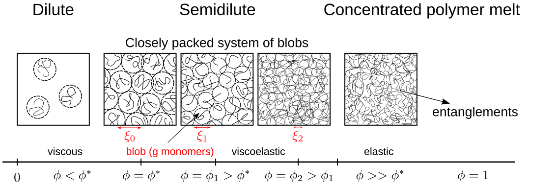
Due to the overlap of the chains in the semidilute regime, there must be some length scale \(\xi\) (called correlation length),such that
- for \(r<\xi\) the monomers are just surrounded by solvent mostly or same chain monomers
- for \(r>\xi\) the monomer starts to see other chains
This correlation length helps us to subdivide the chain into blobs of a size \(\xi\). This size is determined by the free volume and the chain size again via
\[ \xi \approx b \left ( \frac{\nu}{b^3}\right )^{2\nu-1} g^{\nu} \]
with \(g\) segments in the blob. The correlation volume is then given by \(\phi=gb^3/\xi^3\) such that we can express the blob size as
\[ \xi \approx b\phi^{-\frac{\nu}{3\nu-1}} \begin{cases}\phi^{-1}\,&\text{for }\nu=1/2\\ \phi^{-3/4}\,&\text{for }\nu=3/5\end{cases} \]
From this, the number of segements per blob follow to scale as
\[ g\approx \phi^{-\frac{1}{3\nu-1}} \]
Since for \(r>\xi\) the monomers sees other chains, excluded volume interactions are screened. Thus, a semidilute solution of polymer is like a “melt” of blobs. The blobs are the new segments of a random walk of the size
\[ R\approx \xi \left ( \frac{N}{g}\right )^{1/2}\approx bN^{1/2}\phi^{-\frac{2\nu-1}{6\nu-2}}\begin{cases} \phi^{0}\, & \text{for }\nu=1/2\\ \phi^{-1/8}\, & \text{for }\nu=3/5 \end{cases} \]
The polymer size therefore changes only very weakly with the concentration. To understand the dynamics of these polymer solutions, we now need the two models we have refered to already earlier
- Zimm model which was valid for a dilute solution where monomers are hydrodynamically coupled
- Rouse model which typically is valid in a melt in the absence of entanglements and neglects hydrodynamic coupling
Since there is a characteristic length scale in the structure of the semidilute solutions, the hydrodynamic coupling must also possess a characteristic length scale \(\xi_h\) such that
- when \(r<\xi_h\) the segments are coupled by hydrodynamics and the Zimm model can be applied
- when \(r>\xi_h\) the hydrodynamics is screened and the system is comparable to a melt of blobs
In fact, this hydrodynamic length scale is assumed to be the same as the structural length scale \(\xi_h=\xi\) such that we have for the short length scales
Zimm dynamics
Here the chain sections feel the hydrodynamic coupling which leads to a maximum relaxation time
\[ \tau_{\xi}\approx \frac{\eta_s \xi^{3}}{k_B T}\approx \frac{\eta_s b^{}3}{k_B T}\phi^{-\frac{3\nu}{3\nu-1}} \]
as already used earlier. Beyond this length scale the dynamics becomes Rouse like and we have the
Rouse dynamics
with the longest relaxation time being for the whole chain of blobs
\[ \tau_{chain}\approx \tau_{\xi}\left ( \frac{N}{g}\right )^{2}\approx \frac{\eta_s b^{3}}{k_B T}N^2 \phi^{\frac{2-3\nu}{3\nu-1}} \]
scaling as
\[ \tau_{chain}\approx \begin{cases} \phi\, & \text{for } \nu=1/2\\ \phi^{0.31}\, & \text{for } \nu=3/5 \end{cases} \]
with the concentration of the chain \(\phi\). With this longest relaxation time for the chain we can now obtain the diffusion coefficient of a chain in the semi-dilute regime, which is
\[ D\approx \frac{R^2}{\tau_{chain}}\approx \frac{k_B T}{\eta_s b N} \phi^{-\frac{1-\nu}{3\nu -1}}\approx D_{z}\left (\frac{\phi}{\phi^{*}}\right )^{-\frac{1-\nu}{3\nu-1}} \]
with \(D_z=k_B T/\eta_s b N^{\nu}\). The diffusion coefficient therefore scales as
\[ D\approx \begin{cases} \phi^{0}\, & \text{for } \nu=1/2\\ \phi^{-0.54}\, & \text{for } \nu=3/5 \end{cases} \]
This scaling for the real chain with an exponent of \(-0.54\) is also found in the experiments.
insert experimetal image
33.0.1 Stress Relaxation
The stress relaxation now follows the dynamics in the two regimes and can be obtained from the correponding relaxation time spectrum as we have introduced that also already earlier.
For \(\tau_0<t<\tau_{\xi}\):
\[ G(t)\approx \frac{k_B T}{b^3}\phi \left ( \frac{t}{\tau_0}\right )^{-\frac{1}{3\nu}} \]
For \(\tau_{\xi}<t<\tau_{chain}\):
\[ G(t)\approx \frac{k_B T}{b^3}\phi^{\frac{3\nu}{3\nu-1}} \left ( \frac{t}{\tau_0}\right )^{-\frac{1}{2}} \]