Introduction to Numerical Integration in Physics

Numerical integration stands as one of the fundamental computational tools in physics, enabling us to solve problems where analytical solutions are either impossible or impractical. In physics, we frequently encounter integrals when calculating quantities such as:

• Work done by a variable force
• Electric and magnetic fields from complex charge distributions
• Center of mass of irregularly shaped objects
• Probability distributions in quantum mechanics
• Energy levels in quantum wells with arbitrary potentials
• Heat flow in non-uniform materials

The need for numerical integration arises because many physical systems are described by functions that cannot be integrated analytically. For example, the potential energy of a complex molecular system, the trajectory of a spacecraft under multiple gravitational influences, or the behavior of quantum particles in complex potentials.

In this lecture, we’ll explore three progressively more accurate numerical integration methods: the Box method, Trapezoid method, and Simpson’s method. We’ll analyze their accuracy, efficiency, and appropriate applications in physical problems.

Box Method (Rectangle Method)

Theory and Implementation

Figure 1: Box Method Illustration

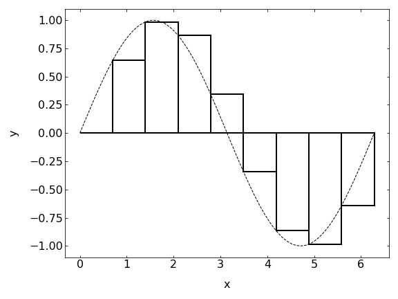
The Box method (also known as the Rectangle method) represents the simplest approach for numerical integration. It approximates the function in each interval \(\Delta x\) with a constant value taken at a specific point of the interval—typically the left endpoint, although midpoint or right endpoint variants exist.

Mathematically, the definite integral is approximated as:

\[\begin{equation} \int_{a}^{b} f(x) dx \approx \sum_{i=1}^{N} f(x_{i}) \Delta x \end{equation}\]

Where:

• \(a\) and \(b\) are the integration limits
• \(N\) is the number of intervals
• \(\Delta x = \frac{b-a}{N}\) is the width of each interval
• \(x_i\) represents the left endpoint of each interval

The method gets its name from the visual representation of the approximation as a series of rectangular boxes.

Box Method Applications

Physics Application: Work Calculation

Consider a particle moving along a straight line under a variable force \(F(x) = kx^2\) where \(k\) is some constant. The work done by this force when moving the particle from position \(x=0\) to \(x=L\) is given by:

\[\begin{equation} W = \int_{0}^{L} F(x) dx = \int_{0}^{L} kx^2 dx \end{equation}\]

We can approximate this integral using the Box method, particularly useful when the force follows a complex pattern measured at discrete points.

Convergence Analysis

Trapezoid Method

Theory and Implementation

Figure 2: Trapezoid Method Illustration

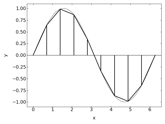
The Trapezoid method improves upon the Box method by approximating the function with linear segments between consecutive points. Instead of using constant values within each interval, it connects adjacent points with straight lines, forming trapezoids.

The mathematical formula for the Trapezoid method is:

\[\begin{equation} \int_{a}^{b} f(x) dx \approx \sum_{i=1}^{N-1} \frac{f(x_i) + f(x_{i+1})}{2} \Delta x \end{equation}\]

Where: - \(\Delta x = \frac{b-a}{N-1}\) is the width of each interval - \(x_i\) are the sample points

This method is particularly effective for smoothly varying functions, which are common in physical systems.

Trapezoid Application

Physics Application: Electric Potential from Charge Distribution

A practical application in electromagnetism involves calculating the electric potential at a point due to a non-uniform charge distribution along a line. For a linear charge density \(\lambda(x)\) along the x-axis, the potential at point \((0,d)\) is given by:

\[\begin{equation} V(0,d) = \frac{1}{4\pi\epsilon_0} \int_{a}^{b} \frac{\lambda(x)}{\sqrt{x^2 + d^2}} dx \end{equation}\]

The Trapezoid method is well-suited for this calculation, especially when \(\lambda(x)\) is provided as experimental data points.

Convergence Analysis

Simpson’s Method

Theory and Implementation

Figure 3: Simpson’s Method Illustration

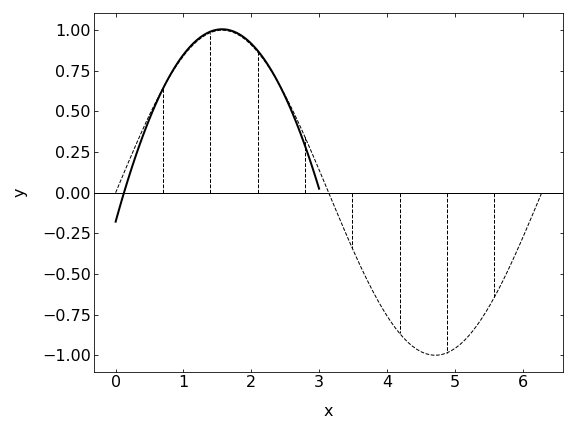
Simpson’s method represents a significant improvement in accuracy over the previous methods by approximating the function with parabolic segments rather than straight lines. This approach is particularly effective for functions with curvature, which are ubiquitous in physics problems.

The mathematical formulation of Simpson’s rule is:

\[\begin{equation} \int_{a}^{b} f(x) dx \approx \frac{\Delta x}{3} \sum_{i=0}^{(N-1)/2} \left(f(x_{2i}) + 4f(x_{2i+1}) + f(x_{2i+2})\right) \end{equation}\]

Where: - \(N\) is the number of intervals (must be even) - \(\Delta x = \frac{b-a}{N}\) is the width of each interval

Simpson’s rule is derived from fitting a quadratic polynomial through every three consecutive points and then integrating these polynomials.

Simpson’s Nethod Applications

Physics Application: Quantum Mechanical Probability

A fundamental application in quantum mechanics involves calculating the probability of finding a particle in a region of space. For a wavefunction \(\psi(x)\), the probability of finding the particle between positions \(a\) and \(b\) is:

\[\begin{equation} P(a \leq x \leq b) = \int_{a}^{b} |\psi(x)|^2 dx \end{equation}\]

Simpson’s method provides high accuracy for these calculations, especially important when dealing with oscillatory wavefunctions.

Convergence Analysis

Simpson’s Rule for Numerical Integration

Simpson’s Rule is a method for numerical integration that approximates the definite integral of a function by using quadratic polynomials.

1. For an integral \(\int_a^b f(x)dx\), Simpson’s Rule fits a quadratic function through three points:

   • \(f(a)\)
   • \(f(\frac{a+b}{2})\)
   • \(f(b)\)

2. Let’s define:

   • \(h = \frac{b-a}{2}\)
   • \(x_0 = a\)
   • \(x_1 = \frac{a+b}{2}\)
   • \(x_2 = b\)

3. The quadratic approximation has the form: \[P(x) = Ax^2 + Bx + C\]

4. This polynomial must satisfy: \[f(x_0) = Ax_0^2 + Bx_0 + C\] \[f(x_1) = Ax_1^2 + Bx_1 + C\] \[f(x_2) = Ax_2^2 + Bx_2 + C\]

5. Using Lagrange interpolation: \[P(x) = f(x_0)L_0(x) + f(x_1)L_1(x) + f(x_2)L_2(x)\]

   where \(L_0\), \(L_1\), \(L_2\) are the Lagrange basis functions.

Final Formula

The integration of this polynomial leads to Simpson’s Rule:

\[\int_a^b f(x)dx \approx \frac{h}{3}[f(a) + 4f(\frac{a+b}{2}) + f(b)]\]

Error Term

The error in Simpson’s Rule is proportional to:

\[-\frac{h^5}{90}f^{(4)}(\xi)\]

for some \(\xi \in [a,b]\)

Composite Simpson’s Rule

For better accuracy, we can divide the interval into \(n\) subintervals (where \(n\) is even):

\[\int_a^b f(x)dx \approx \frac{h}{3}[f(x_0) + 4\sum_{i=1}^{n/2}f(x_{2i-1}) + 2\sum_{i=1}^{n/2-1}f(x_{2i}) + f(x_n)]\]

where \(h = \frac{b-a}{n}\)

The method is particularly effective for integrating functions that can be well-approximated by quadratic polynomials over small intervals.

When to Use Each Method

Choosing the appropriate numerical integration method for a physics problem requires consideration of several factors:

Method	Error Order	Optimal For	Limitations	Example Physics Applications
Box	\(O(N^{-1})\)	- Simple, rapid calculations - Step functions - Real-time processing - Discontinuous functions	- Low accuracy - Requires many points for decent results	- Basic data analysis - Signals with sharp transitions - First approximations in mechanics
Trapezoid	\(O(N^{-2})\)	- Smooth, continuous functions - Moderate accuracy requirements - Periodic functions	- Struggles with sharp peaks - Not ideal for higher derivatives	- Electric and magnetic fields - Orbital mechanics - Path integrals - Work/energy calculations
Simpson	\(O(N^{-4})\)	- Functions with significant curvature - High precision requirements - Oscillatory integrands	- More computationally intensive - Requires evenly spaced points	- Quantum mechanical probabilities - Wave optics - Statistical mechanics - Thermal physics

Additional Considerations

• Adaptive methods can be more efficient when dealing with functions that have varying behavior across the integration range
• Improper integrals (with infinite limits or singularities) often require specialized techniques beyond these basic methods
• Higher-dimensional integration problems (common in statistical and quantum mechanics) may benefit from Monte Carlo methods rather than these quadrature rules

Error Analysis

The error behavior of numerical integration methods is crucial for understanding their applicability to physics problems:

• Box Method: Error \(\propto\) \(O(\Delta x)\) = \(O(N^{-1})\) (linear convergence)
  • The error is proportional to the step size
  • The dominant error term comes from the first derivative of the function
• Trapezoid Method: Error \(\propto\) \(O(\Delta x^2)\) = \(O(N^{-2})\) (quadratic convergence)
  • The error is proportional to the square of the step size
  • The dominant error term involves the second derivative of the function
• Simpson’s Method: Error \(\propto\) \(O(\Delta x^4)\) = \(O(N^{-4})\) (fourth-order convergence)
  • The error is proportional to the fourth power of the step size
  • The dominant error term involves the fourth derivative of the function

Consequently, if we double the number of points:

• Box method: error reduced by a factor of 2
• Trapezoid method: error reduced by a factor of 4
• Simpson’s method: error reduced by a factor of 16

The practical impact of these convergence rates is substantial. For example, to achieve an error of \(10^{-6}\) for a well-behaved function:

• Box method might require millions of points
• Trapezoid method might require thousands of points
• Simpson’s method might require only hundreds of points

This explains why higher-order methods are generally preferred for physics applications requiring high precision, such as quantum mechanical calculations, gravitational wave analysis, or computational fluid dynamics.

Conclusion

Numerical integration stands as a cornerstone of computational physics, bridging the gap between theoretical models and practical analysis of real-world systems. In this lecture, we’ve explored three fundamental methods—Box, Trapezoid, and Simpson’s method—that provide different balances of simplicity, accuracy, and computational efficiency.

The key insights from our study include:

1. Method selection matters: The choice of integration technique can dramatically impact both accuracy and computational efficiency. For typical physics applications requiring high precision, Simpson’s method often provides the optimal balance of accuracy and computation cost.

2. Error scaling: Understanding how errors scale with the number of sampling points is crucial for reliable scientific computation. The higher-order convergence of Simpson’s method (\(O(N^{-4})\)) makes it particularly valuable for precision-critical applications in physics.

3. Physical context: The nature of the underlying physical system should guide your choice of numerical method. Smoothly varying functions benefit from higher-order methods, while functions with discontinuities may require adaptive or specialized approaches.

4. Verification: Always verify numerical results against analytical solutions when possible, or compare results from different numerical methods with increasing resolution to establish confidence in your calculations.

As you progress in your physics education, these numerical integration techniques will become essential tools in your computational toolkit, enabling you to tackle increasingly complex physical systems from quantum mechanics to astrophysics, fluid dynamics, and beyond.

In advanced courses, you’ll explore additional techniques such as Gaussian quadrature, Romberg integration, and specialized methods for oscillatory, singular, or multi-dimensional integrals—each designed to address specific challenges encountered in modern physics.

Remember that numerical integration is not merely a computational technique but a powerful approach to understanding physical systems that resist analytical treatment, making it an indispensable skill for the modern physicist.

Advanced Topics in Numerical Integration

Adaptive Integration Methods

The methods we’ve discussed so far use equal spacing between sampling points. However, most real-world physics problems involve functions that vary dramatically across the integration range. Adaptive methods adjust the point distribution to concentrate more points where the function changes rapidly.

Multi-dimensional Integration

Many physics problems require integration over multiple dimensions, such as calculating mass moments of inertia, electric fields from volume charge distributions, or statistical mechanics partition functions.

For 2D integration, we can extend our 1D methods using the concept of iterated integrals:

\[\begin{equation} \int_{a}^{b}\int_{c}^{d} f(x,y) dy dx \approx \sum_{i=1}^{N_x} \sum_{j=1}^{N_y} w_i w_j f(x_i, y_j) \end{equation}\]

Where \(w_i\) and \(w_j\) are the weights for the respective 1D methods.

Monte Carlo Integration

For higher-dimensional integrals and complex domains, Monte Carlo methods become increasingly efficient. These methods use random sampling to approximate integrals and are particularly valuable in quantum and statistical physics.

Application to Real Physics Problems

Let’s examine two common scenarios in physics that benefit from numerical integration:

1. Non-uniform Magnetic Field: When a charged particle moves through a non-uniform magnetic field, the work done can be calculated as:

   \[W = q\int_{\vec{r}_1}^{\vec{r}_2} \vec{v} \times \vec{B}(\vec{r}) \cdot d\vec{r}\]

2. Quantum Tunneling: The tunneling probability through a potential barrier is given by:

   \[T \approx \exp\left(-\frac{2}{\hbar}\int_{x_1}^{x_2} \sqrt{2m(V(x) - E)}\, dx\right)\]

In both cases, the integrals frequently cannot be solved analytically due to the complex spatial dependence of the fields or potentials, making numerical integration indispensable for modern physics.