Solving Ordinary Differential Equations

Introduction

In the previous lecture on numerical differentiation, we explored how to compute derivatives numerically using finite difference methods and matrix representations. We learned that:

Finite difference approximations allow us to estimate derivatives at discrete points
Differentiation can be represented as matrix operations
The accuracy of these approximations depends on the order of the method and step size

Building on this foundation, we can now tackle one of the most important applications in computational physics: solving ordinary differential equations (ODEs). Almost all dynamical systems in physics are described by differential equations, and learning how to solve them numerically is essential for modeling physical phenomena.

As second-semester physics students, you’ve likely encountered differential equations in various contexts:

Newton’s second law: \(F = ma = m\frac{d^2x}{dt^2}\)
Simple harmonic motion: \(\frac{d^2x}{dt^2} + \omega^2x = 0\)
RC circuits: \(\frac{dQ}{dt} + \frac{1}{RC}Q = 0\)
Heat diffusion: \(\frac{\partial T}{\partial t} = \alpha \nabla^2 T\)

While analytical solutions exist for some simple cases, real-world physics problems often involve complex systems where analytical solutions are either impossible or impractical to obtain. This is where numerical methods become indispensable tools for the working physicist.

Types of ODE Solution Methods

There are two main approaches to solving ODEs numerically:

Implicit methods: These methods solve for all time points simultaneously using matrix operations. They treat the problem as a large system of coupled algebraic equations. Just as you might solve a system of linear equations \(Ax = b\) in linear algebra, implicit methods set up and solve a larger matrix equation that represents the entire evolution of the system.
Explicit methods: These methods march forward in time, computing the solution step by step. Starting from the initial conditions, they use the current state to calculate the next state, similar to how you might use the position and velocity at time \(t\) to predict the position and velocity at time \(t + \Delta t\).

We’ll explore both approaches, highlighting their strengths and limitations. Each has its place in physics: implicit methods often handle “stiff” problems better (problems with vastly different timescales), while explicit methods are typically easier to implement and can handle nonlinear problems more naturally.

The Harmonic Oscillator: A Prototypical ODE

Physics Interlude: The Harmonic Oscillator

The harmonic oscillator is one of the most fundamental systems in physics, appearing in mechanics, electromagnetism, quantum mechanics, and many other fields. It serves as an excellent test case for ODE solvers due to its simplicity and known analytical solution.

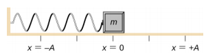
The harmonic oscillator describes any system that experiences a restoring force proportional to displacement. Physically, this occurs in:

A mass on a spring (Hooke’s law: \(F = -kx\))
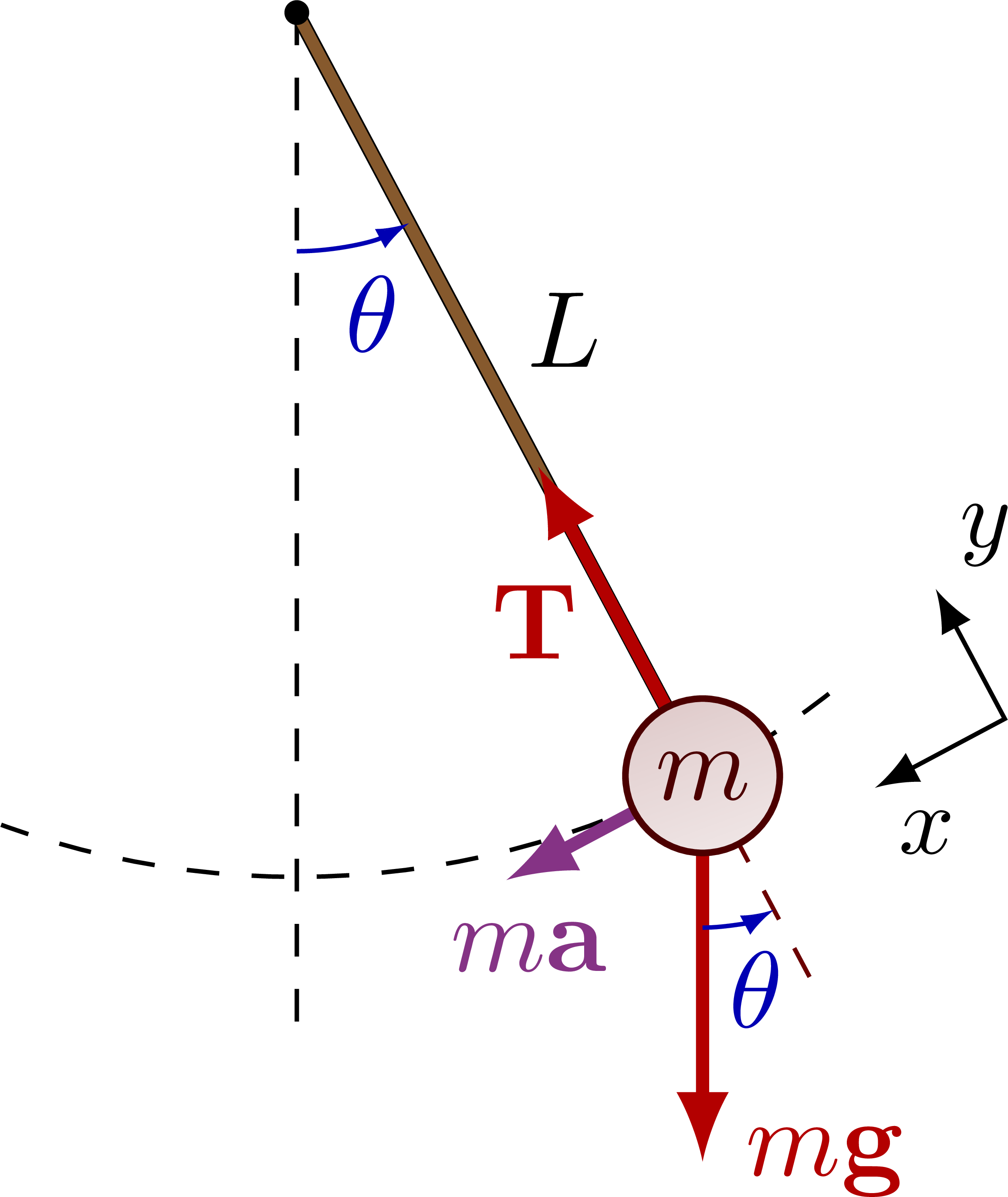
A pendulum for small angles (where \(\sin\theta \approx \theta\))
An LC circuit with inductors and capacitors
Molecular vibrations in chemistry
Phonons in solid state physics

Figure 1: A mass suspended from a spring demonstrates a classic harmonic oscillator. When displaced from equilibrium, the spring exerts a restoring force proportional to the displacement, leading to oscillatory motion.

The equation of motion for a classical harmonic oscillator is:

\[\begin{equation} \frac{d^2x}{dt^2} + \omega^2 x = 0 \end{equation}\]

where \(\omega = \sqrt{k/m}\) is the angular frequency, with \(k\) being the spring constant and \(m\) the mass. In terms of Newton’s second law, this is: \[\begin{equation} m\frac{d^2x}{dt^2} = -kx \end{equation}\]

This second-order differential equation requires two initial conditions: - Initial position: \(x(t=0) = x_0\) - Initial velocity: \(\dot{x}(t=0) = v_0\)

The analytical solution is: \[\begin{equation} x(t) = x_0 \cos(\omega t) + \frac{v_0}{\omega} \sin(\omega t) \end{equation}\]

This represents sinusoidal oscillation with a constant amplitude and period \(T = 2\pi/\omega\). The total energy of the system (kinetic + potential) remains constant: \[\begin{equation} E = \frac{1}{2}mv^2 + \frac{1}{2}kx^2 \end{equation}\]

This energy conservation will be an important test for our numerical methods.

Implicit Matrix Solution

Using the matrix representation of the second derivative operator from our previous lecture, we can transform the ODE into a linear system that can be solved in one step. This approach treats the entire time evolution as a single mathematical problem.

Setting Up the System

From calculus, we know that the second derivative represents the rate of change of the rate of change. Physically, this corresponds to acceleration in mechanics. In numerical terms, we need to approximate this using finite differences.

Recall that we can represent the second derivative operator as a tridiagonal matrix:

\[D_2 = \frac{1}{\Delta t^2} \begin{bmatrix} -2 & 1 & 0 & 0 & \cdots & 0\\ 1 & -2 & 1 & 0 & \cdots & 0\\ 0 & 1 & -2 & 1 & \cdots & 0\\ \vdots & \vdots & \vdots & \vdots & \ddots & \vdots\\ 0 & \cdots & 0 & 1 & -2 & 1\\ 0 & \cdots & 0 & 0 & 1 & -2\\ \end{bmatrix}\]

This matrix implements the central difference approximation for the second derivative: \[\begin{equation} \frac{d^2x}{dt^2} \approx \frac{x_{i+1} - 2x_i + x_{i-1}}{\Delta t^2} \end{equation}\]

Each row in this matrix corresponds to the equation for a specific time point, linking it to its neighbors.

The harmonic oscillator term \(\omega^2 x\) represents the restoring force. In a spring system, this is \(F = -kx\) divided by mass, giving \(a = -\frac{k}{m}x = -\omega^2 x\). This can be represented by a diagonal matrix:

\[V = \omega^2 I = \omega^2 \begin{bmatrix} 1 & 0 & 0 & \cdots & 0\\ 0 & 1 & 0 & \cdots & 0\\ 0 & 0 & 1 & \cdots & 0\\ \vdots & \vdots & \vdots & \ddots & \vdots\\ 0 & 0 & 0 & \cdots & 1\\ \end{bmatrix}\]

Our equation \(\frac{d^2x}{dt^2} + \omega^2 x = 0\) becomes the matrix equation \((D_2 + V)x = 0\), where \(x\) is the vector containing the positions at all time points \((x_1, x_2, ..., x_n)\). This is a large system of linear equations that determine the entire trajectory at once.

Incorporating Initial Conditions

To solve this system, we need to incorporate the initial conditions by modifying the first rows of our matrix. This is a crucial step because a second-order differential equation needs two initial conditions to define a unique solution. In physical terms, we need to know both the initial position (displacement) and the initial velocity of our oscillator. We incorporate these conditions directly into our matrix equation:

\[M = \begin{bmatrix} \color{red}{1} & \color{red}{0} & \color{red}{0} & \color{red}{0} & \color{red}{\cdots} & \color{red}{0} \\ \color{blue}{-1} & \color{blue}{1} & \color{blue}{0} & \color{blue}{0} & \color{blue}{\cdots} & \color{blue}{0} \\ \frac{1}{\Delta t^2} & -\frac{2}{\Delta t^2}+\omega^2 & \frac{1}{\Delta t^2} & 0 & \cdots & 0 \\ 0 & \frac{1}{\Delta t^2} & -\frac{2}{\Delta t^2}+\omega^2 & \frac{1}{\Delta t^2} & \cdots & 0 \\ \vdots & \vdots & \vdots & \vdots & \ddots & \vdots \\ 0 & \cdots & 0 & \frac{1}{\Delta t^2} & -\frac{2}{\Delta t^2}+\omega^2 & \frac{1}{\Delta t^2} \\ \end{bmatrix}\]

The first row (in red) enforces \(x(0) = x_0\) (initial position), and the second row (in blue) implements the initial velocity condition. The rest of the matrix represents the differential equation at each time step. By incorporating the initial conditions directly into the matrix, we ensure that our solution satisfies both the differential equation and the initial conditions.

This matrix-based approach has several advantages:

It solves for all time points simultaneously, giving the entire trajectory in one operation
It can be very stable for certain types of problems, particularly “stiff” equations
It handles boundary conditions naturally by incorporating them into the matrix structure
It often provides good energy conservation for oscillatory systems

However, it also has limitations:

It requires solving a large linear system, which becomes computationally intensive for long simulations
It’s not suitable for nonlinear problems without modification (e.g., a pendulum with large angles where \(\sin\theta \neq \theta\))
Memory requirements grow with the time span (an N×N matrix for N time steps)
Implementing time-dependent forces is more complex than with explicit methods

From a physics perspective, this approach is similar to finding stationary states in quantum mechanics or solving boundary value problems in electrostatics—we’re solving the entire system at once rather than stepping through time.

Explicit Numerical Integration Methods

An alternative approach is to use explicit step-by-step integration methods. These methods convert the second-order ODE to a system of first-order ODEs and then advance the solution incrementally, similar to how we intuitively understand physical motion: position changes based on velocity, and velocity changes based on acceleration.

Converting to a First-Order System

To convert our second-order ODE to a first-order system, we introduce a new variable \(v = dx/dt\) (the velocity):

\[\begin{align} \frac{dx}{dt} &= v \\ \frac{dv}{dt} &= -\omega^2 x \end{align}\]

This transformation is common in physics. For example, in classical mechanics, we often convert Newton’s second law (a second-order ODE) into phase space equations involving position and momentum. In the case of the harmonic oscillator:

The first equation simply states that the rate of change of position is the velocity
The second equation comes from \(F = ma\) where \(F = -kx\), giving \(a = \frac{F}{m} = -\frac{k}{m}x = -\omega^2 x\)

We can now represent the state of our system as a vector

\[\vec{y} = \begin{bmatrix} x \\ v \end{bmatrix}\]

and the derivative as

\[\dot{\vec{y}} = \begin{bmatrix} v \\ -\omega^2 x \end{bmatrix}\]

This representation is called the “phase space” description, and is fundamental in classical mechanics and dynamical systems theory.

Recipe to solve a differential equation

State your differential equation as a system of ordinary differential equations \[\dot{\vec{y}} = \begin{bmatrix} v \\ -\omega^2 x \end{bmatrix}\]

Write a function that represents you physical system

def SHO(time, state, omega=2):
    g0 = state[1]               ->velocity
    g1 = -omega * state [0]       ->acceleration
    return np.array([g0, g1])

Use a function to integrate the system of ODEs

t_euler, y_euler = euler_method(lambda t, y: SHO(t, y, omega),
    y0,
    t_span,
    dt
)

solution = solve_ivp( lambda t, y: SHO(t, y, omega),
    t_span,
    y0,
    method='BDF',
    t_eval=t_eval
)

The simplest explicit integration method is the Euler method, derived from the first-order Taylor expansion:

\[\begin{equation} \vec{y}(t + \Delta t) \approx \vec{y}(t) + \dot{\vec{y}}(t) \Delta t \end{equation}\]

This is essentially a linear approximation—assuming the derivative stays constant over the small time step. Physically, it’s like assuming constant velocity when updating position, and constant acceleration when updating velocity over each small time interval.

For the harmonic oscillator, this becomes:

\[\begin{align} x_{n+1} &= x_n + v_n \Delta t \\ v_{n+1} &= v_n - \omega^2 x_n \Delta t \end{align}\]

The physical interpretation is straightforward:

The new position equals the old position plus the displacement (velocity × time)
The new velocity equals the old velocity plus the acceleration (-ω²x) multiplied by the time step

In practice, the Euler method will cause the total energy of a harmonic oscillator to increase over time, which is physically incorrect. This is because the method doesn’t account for the continuous change in acceleration during the time step.

The Euler method often performs poorly for oscillatory systems, as it tends to artificially increase the energy over time. A simple but effective improvement is the Euler-Cromer method (also known as the symplectic Euler method), which uses the updated velocity for the position update:

\[\begin{align} v_{n+1} &= v_n - \omega^2 x_n \Delta t \\ x_{n+1} &= x_n + v_{n+1} \Delta t \end{align}\]

Notice the subtle but crucial difference: we use \(v_{n+1}\) (the newly calculated velocity) to update the position, rather than \(v_n\).

This small change dramatically improves energy conservation for oscillatory systems. From a physics perspective, this method better preserves the structure of Hamiltonian systems, which include the harmonic oscillator, planetary motion, and many other important physical systems.

The Euler-Cromer method is especially valuable in physics simulations where long-term energy conservation is important, such as:

Orbital mechanics
Molecular dynamics
Plasma physics
N-body simulations

While not perfect, this simple modification makes the method much more useful for real physical systems with oscillatory behavior.

For higher accuracy, we can use the midpoint method (also known as the second-order Runge-Kutta method or RK2). This evaluates the derivative at the midpoint of the interval, providing a better approximation of the average derivative over the time step.

\[\begin{align} k_1 &= f(t_n, y_n) \\ k_2 &= f(t_n + \frac{\Delta t}{2}, y_n + \frac{\Delta t}{2}k_1) \\ y_{n+1} &= y_n + \Delta t \cdot k_2 \end{align}\]

The physical intuition behind this method is:

First, calculate the initial derivative \(k_1\) (representing the initial rates of change)
Use this derivative to estimate the state at the middle of the time step
Calculate a new derivative \(k_2\) at this midpoint
Use the midpoint derivative to advance the full step

This is analogous to finding the average velocity by looking at the velocity in the middle of a time interval, rather than just at the beginning. In physical problems with continuously varying forces, this provides a much better approximation than the Euler method.

The midpoint method achieves \(O(\Delta t^2)\) accuracy, meaning the error decreases with the square of the step size. This makes it much more accurate than Euler’s method for the same computational cost.

Comparing the Methods

Let’s compare these methods for the harmonic oscillator:

Observations:

Euler Method: Simple but least accurate. It systematically increases the total energy of the system, causing the amplitude to grow over time.
Euler-Cromer Method: Much better energy conservation for oscillatory systems with minimal additional computation.
Midpoint Method: Higher accuracy and better energy conservation.

The choice of method depends on the specific requirements of your problem:

Use Euler for simplicity when accuracy is not critical
Use Euler-Cromer for oscillatory systems when computational efficiency is important
Use Midpoint or higher-order methods when accuracy is crucial

Advanced Methods with SciPy

For practical applications, SciPy provides sophisticated ODE solvers with adaptive step size control, error estimation, and specialized algorithms for different types of problems. These methods represent the state-of-the-art in numerical integration and are what working physicists typically use for research and advanced applications.

What Makes These Methods Advanced?

Adaptive Step Size: Unlike our fixed-step methods, these solvers can automatically adjust the step size based on the local error estimate, taking smaller steps where the solution changes rapidly and larger steps where it’s smooth.
Higher-Order Methods: These solvers use higher-order approximations (4th, 5th, or even 8th order), achieving much higher accuracy with the same computational effort.
Error Control: They can maintain the error below a specified tolerance, giving you confidence in the accuracy of your results.
Specialized Methods: Different methods are optimized for different types of problems (stiff vs. non-stiff, conservative vs. dissipative).

Using solve_ivp for the Harmonic Oscillator

Advanced Example: Damped Driven Pendulum

Let’s apply these methods to a more complex system: a damped driven pendulum. This system can exhibit chaotic behavior under certain conditions, making it a fascinating study in nonlinear dynamics.

Figure 2: The damped driven pendulum. External driving forces and damping (friction) create a system that can exhibit complex behaviors from regular oscillations to chaos.

Physical Context

The damped driven pendulum represents many real physical systems

A physical pendulum with friction and external driving force
An RLC circuit with nonlinear components
Josephson junctions in superconductivity
Certain types of mechanical and electrical oscillators

The equation of motion is:

\[\begin{equation} \frac{d^2\theta}{dt^2} + b\frac{d\theta}{dt} + \omega_0^2\sin\theta = F_0\cos(\omega_d t) \end{equation}\]

where

\(\theta\) is the angle from vertical (radians)
\(b\) is the damping coefficient (represents friction or resistance)
\(\omega_0 = \sqrt{g/L}\) is the natural frequency (where \(g\) is gravity and \(L\) is pendulum length)
\(F_0\) is the driving amplitude (strength of the external force)
\(\omega_d\) is the driving frequency (how rapidly the external force oscillates)

This equation differs from the harmonic oscillator in three crucial ways:

The \(\sin\theta\) term (rather than just \(\theta\)) makes it nonlinear
The damping term \(b\frac{d\theta}{dt}\) causes energy dissipation
The driving term \(F_0\cos(\omega_d t)\) adds energy to the system

These additions make the system much more realistic and rich in behavior. Students could explore this system by varying parameters like the damping coefficient (b), driving amplitude (F0), and driving frequency (omega_d) to observe how the pendulum transitions between regular oscillations, period doubling, and chaos.

Exploring Chaotic Behavior

Chaotic motion refers to a deterministic system whose behavior appears random and exhibits extreme sensitivity to initial conditions—the famous “butterfly effect.” In the damped driven pendulum, chaos emerges when the system’s nonlinear restoring force (\(\sin\theta\) term) interacts with sufficient driving force. For this system, chaotic behavior typically appears when the driving amplitude \(F_0\) exceeds a critical value (approximately 1.0 in our case) while maintaining moderate damping (\(b \approx 0.1\)) and a driving frequency \(\omega_d\) that is not too far from the natural frequency \(\omega_0\). In the chaotic regime, the pendulum’s trajectory becomes unpredictable over long time scales, despite being governed by deterministic equations. The phase space transforms from closed orbits (regular motion) to a strange attractor with fractal structure, and the system never settles into a periodic oscillation.

Lyapunov Exponents: Quantifying Chaos

The Lyapunov exponent is a powerful mathematical tool for characterizing chaotic systems. It measures the rate at which nearby trajectories in phase space diverge over time. For a system with state vector \(\vec{x}\), if two initial conditions differ by a small displacement \(\delta\vec{x}_0\), then after time \(t\), this separation grows approximately as:

\[|\delta\vec{x}(t)| \approx e^{\lambda t}|\delta\vec{x}_0|\]

where \(\lambda\) is the Lyapunov exponent.

A positive Lyapunov exponent (\(\lambda > 0\)) indicates chaos: nearby trajectories diverge exponentially, making long-term prediction impossible. The larger the exponent, the more chaotic the system.
A zero Lyapunov exponent (\(\lambda = 0\)) suggests a stable limit cycle or quasiperiodic behavior.
A negative Lyapunov exponent (\(\lambda < 0\)) indicates a stable fixed point, where trajectories converge.

For our damped driven pendulum, we can numerically estimate the Lyapunov exponent by comparing how two slightly different initial conditions evolve over time. For instance, we might begin with two pendulums at nearly the same angle—perhaps \(\theta_1(0) = 0.1\) and \(\theta_2(0) = 0.1001\)—while keeping their initial angular velocities identical at \(\omega_1(0) = \omega_2(0) = 0\). As we simulate both systems, we can track the separation between their trajectories in phase space. This separation represents the difference vector \(\delta\vec{x}(t) = [\theta_2(t) - \theta_1(t), \omega_2(t) - \omega_1(t)]\). Initially, this difference is very small, but in a chaotic system, it grows exponentially with time. By measuring this growth rate, we can compute the Lyapunov exponent as \(\lambda \approx \frac{1}{t}\ln\left(\frac{|\delta\vec{x}(t)|}{|\delta\vec{x}(0)|}\right)\). When examining our pendulum system, which has two dimensions (\(\theta\) and \(\omega\)), we actually have two Lyapunov exponents forming a spectrum. If either of these exponents is positive, we can conclusively determine that our system exhibits chaotic behavior, indicating fundamental unpredictability despite its deterministic nature.

Conclusion

In this lecture, we’ve built upon our knowledge of numerical differentiation to solve ordinary differential equations. We’ve explored:

Implicit Matrix Methods: Using matrices to solve the entire system at once
Explicit Integration Methods: Step-by-step methods like Euler, Euler-Cromer, and Midpoint
Advanced SciPy Methods: Leveraging powerful adaptive solvers for complex problems

Each approach has its strengths and is suited to different types of problems. The matrix method is excellent for linear systems, while explicit methods are more versatile for nonlinear problems. SciPy’s solvers combine accuracy, stability, and efficiency for practical applications.

Physical Relevance

The methods we’ve learned are essential tools for computational physics because they: 1. Allow us to study systems with no analytical solutions 2. Provide insights into nonlinear dynamics and chaos 3. Enable the modeling of realistic systems with friction, driving forces, and complex interactions 4. Connect mathematical formulations with observable physical phenomena

As a second-semester physics student, these numerical tools complement your analytical understanding of mechanics, electromagnetism, and other core physics subjects. When analytical methods reach their limits, these numerical approaches allow you to continue exploring and modeling physical reality.

Exercises

Here are two simple exercises with solutions where you can train your programming skills. In these examples you should use the odeint method from SciPy’s integrate module.

Self-Exercise 1: Simple Harmonic Oscillator

Write a program to solve the equation of motion for a simple harmonic oscillator. This example demonstrates how to solve a second-order differential equation using scipy’s odeint.

The equation of motion is: \(\frac{d^2x}{dt^2} + \omega^2x = 0\)

This represents an idealized spring-mass system or pendulum with small oscillations.

Self-Exercise 2: Damped Driven Harmonic Oscillator using Matrix Method

Model a damped harmonic oscillator with an external driving force using the implicit matrix method. This exercise demonstrates how to solve a second-order differential equation by constructing and solving a matrix system that represents the entire time evolution.

The equation of motion is: \(m\frac{d^2x}{dt^2} + b\frac{dx}{dt} + kx = F_0 \cos(\omega t)\)

Where \(m\) is mass, \(b\) is damping coefficient, \(k\) is spring constant, \(F_0\) is driving amplitude, and \(\omega\) is driving frequency.