Spring Pendulum

In the last lectures, we have explored the use of the scipy module solve_ivp to do the work of solving differential equations for us. We have studied coupled pendula and explored the details of the solutions. This time we have two more projects ahead of us. We first want to consider the motion of a spring pendulum and then come from that to the motion of planets. Both are examples where we have not only a tangential acceleration but also a radial component. Otherwise, these problems do look similar to the ones we considered before.

Physical Model

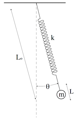
The image below shows the situation we would like to cover in our second project. This is also a kind of coupled pendula, however, the situation is more subtle.

We have a single spring which is mounted to a support and a mass. The spring can be elongated in length but also in angle so that you finally have a pendulum and a spring. Both motions are coupled now in a similar way as for the coupled pendula we treated. This time, however, the length change of the spring modulates the frequency of the pendulum.

Equations of motion

A mass \(m\) is attached to a spring with spring constant \(k\), which is attached to a support point as shown in the figure. The length of the resulting pendulum at any given time is the spring rest length \(L_0\) plus the stretch (or compression) \(L\), and the angle of the pendulum with respect to the vertical is \(\theta\).

The differential equations for this system are given by

\[\begin{eqnarray} \ddot{L}&=&(L_0+L)\dot{\theta}^2-\frac{k}{m}L+g\cos(\theta)\\ \ddot{\theta}&=&-\frac{1}{L_0+L}[g\sin(\theta)+2\dot{L}\dot{\theta}] \end{eqnarray}\]

Let’s break down the terms in these equations:

For the radial motion (L):

\((L_0+L)\dot{\theta}^2\) represents the centrifugal force term
\(-\frac{k}{m}L\) is the restoring force of the spring (Hooke’s law)
\(g\cos(\theta)\) is the component of gravity along the radial direction

For the angular motion (θ):

\(g\sin(\theta)\) represents the gravitational torque
\(2\dot{L}\dot{\theta}\) is the Coriolis force term
The factor \(\frac{1}{L_0+L}\) comes from the moment of inertia

The equations are coupled - the radial and angular motions affect each other. The system shows interesting behavior like:

Energy exchange between radial and angular modes
Non-linear oscillations
Potential for chaotic motion under certain conditions

The key players in this equation are the centrifugal and Coriolis forces. These forces are fictitious forces that arise when we consider the motion of an object in a rotating frame of reference. The centrifugal force is the force that pushes an object away from the center of rotation, while the Coriolis force is the force that acts perpendicular to the direction of motion of an object in a rotating frame.

Centrifugal Force:

\[\begin{equation} \vec{F}_{\text{centrifugal}} = m(\vec{\omega} \times (\vec{\omega} \times \vec{r})) \end{equation}\]

Coriolis Force: \[\begin{equation} \vec{F}_{\text{Coriolis}} = 2m(\vec{\omega} \times \vec{v}_{\text{rel}}) \end{equation}\]

where:

\(m\) is the mass
\(\vec{\omega}\) is the angular velocity vector
\(\vec{r}\) is the position vector
\(\vec{v}_{\text{rel}}\) is the velocity relative to the rotating frame
\(\times\) denotes the cross product

In component form, if we consider rotation about the z-axis with \(\vec{\omega} = \omega\hat{k}\), these become:

Centrifugal Force: \[\begin{equation} \vec{F}_{\text{centrifugal}} = m\omega^2(x\hat{i} + y\hat{j}) \end{equation}\]

Coriolis Force: \[\begin{equation} \vec{F}_{\text{Coriolis}} = 2m\omega(-v_y\hat{i} + v_x\hat{j}) \end{equation}\]

where \(\hat{i}\), \(\hat{j}\), and \(\hat{k}\) are unit vectors in the x, y, and z directions respectively.

Below we write a program that plots the motion of the mass for some initial \(\theta\neq0\). Explore different solutions. We should get that when the spring is very stiff (large k), it reduces approximately to a simple pendulum. When \(\theta\) is small, it can show beats between the spring and pendulum modes.

Numerical Solution

For the numerical solution of the differential equations, we will use the solve_ivp function from the scipy.integrate module. This function provides a more modern and flexible approach to solving initial value problems compared to the older odeint function.

Initial parameters

We will have to think about the initial conditions. We will later modify them to see how the system behaves in different regimes.

Solution

The solution of the differential equations is done by the solve_ivp function.

The solution object contains several attributes. The most important for us is sol.y, which is a 2D array with shape (4, N) where the rows correspond to: 1. The length of the spring (L) 2. The velocity of the spring (dL/dt) 3. The angle of the pendulum (θ) 4. The angular velocity of the pendulum (dθ/dt)

We can convert the solution to the x and y positions of the mass. This is done by the following code. As the length \(L\) is only the elongation of the spring, we have to add the equilibrium length \(L_0\) to get the total length of the spring. The x and y positions are then given by \(L\sin(\theta)\) and \(L\cos(\theta)\).

Plotting

Let’s visualize the motion of our spring pendulum system from several perspectives to gain deeper insights into its dynamics.

Trajectory in Real Space

The first plot shows the physical trajectory of the mass in the x-y plane. This represents the actual path the mass would trace in space as viewed from the side.

Understanding Phase Space

The next plots are what physicists call “phase space” representations. Phase space is a powerful concept in mechanics where we plot a position variable against its corresponding velocity variable. Unlike the real space trajectory, phase space reveals the system’s dynamics in a more fundamental way.

In phase space: - Each point represents both the position and velocity of the system at a given time - Closed curves typically indicate periodic motion - The shape and size of the curves relate to the energy of the system - The conservation of energy often constrains the system to move along specific paths in phase space

Spring Phase Space

This plot shows the spring’s extension L versus its rate of change dL/dt (velocity).

For a simple harmonic oscillator (like a spring with no pendulum), this would produce a perfect ellipse. Deviations from an elliptical shape indicate coupling with the pendulum motion. The area enclosed by the curve is proportional to the energy stored in the spring motion.

Pendulum Phase Space

Similarly, this plot shows the angular position θ versus angular velocity dθ/dt for the pendulum component of the motion.

For a simple pendulum (with no spring), small oscillations would also produce an elliptical phase portrait. The complexity of the curve indicates energy transfer between the pendulum and spring modes. If the curve doesn’t close on itself, it suggests the motion may be quasi-periodic or potentially chaotic.

Energy Exchange Between Modes

The time evolution plot below helps us see how energy transfers between the spring and pendulum modes over time. When the spring amplitude decreases, the pendulum amplitude typically increases, and vice versa, demonstrating energy conservation in the coupled system.

Note that we’ve scaled the angle by a factor of 10 to make the oscillations more visible alongside the spring extension. The beating patterns often visible in this plot are characteristic of coupled oscillators where energy flows back and forth between different modes of the system.