Particle in a box
Let’s apply the whole thing to the problem of a particle in a box. This means, we look at a quantum mechanical object in a potential well.
The problem is sketched below.
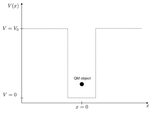
We need to define this rectangular box with zero potential energy inside the box and finite potential energy outside. Since the quantum mechanical object is a wave, we expect that only certain standing waves of particular wavelength can exist inside the box. These waves are connected to certain probability densities of finding the particle at certain positions and specific energy values. These are the energy levels, which are often characteristic of the quantum realm.
Definition of the problem
Before we start, we need to define some quantities:
- we will study a box of d=1 nm in width in a domain of L=10 nm
- we will use N=1001 points for our \(x_{i}\)
- our potential energy shall have a barrier height of 1 eV
- the potential energy inside the box will be zero
Potential energy
We first define the diagonal potential energy matrix. The potential is zero inside the box and V_0 outside.
Kinetic energy
Next we construct the kinetic energy matrix using the finite difference representation of the second derivative.
Hamiltonian and boundary conditions
Finally, we construct the total Hamiltonian operator matrix. For hard wall boundary conditions, we need to ensure that the wavefunction vanishes at the boundaries.
Solution
The last step is to solve the eigenvalue problem using the eigsh method from scipy. We use which='SM' to find the smallest magnitude eigenvalues, which correspond to the lowest energy states.
Plotting the results
Let’s visualize the energy levels and wavefunctions:
The diagram shows the corresponding energy states (the eigenvalues of the solution) and the value \(|\Psi|^2\), which gives the probability to find the particle inside the box. The latter shows that, in contrast to what we expect from classical theory, where we would expect the particle to be with equal probability found at all positions inside the box, we get in quantum mechanics only certain positions at which we would find the particle. Also, the higher the energy state, the more equally is the particle distributed over the box. For a finite box depth, however, we get only a finite number of energy states in which the particle is bound.
A second interesting observation here is that the particle has a finite probability to enter the potential barrier. Especially for the higher energy states, the wavefunction decays exponentially into the barrier. This is similar to the evanescent wave we studied during the last lecture.
Comparison with analytical solution
For an infinite potential well, we can compare our numerical results with the analytical solution. The analytical energy levels for an infinite well are:
\[E_n = \frac{n^2 \pi^2 \hbar^2}{2 m d^2}\]
Let’s compare:
Energies of bound states
In the case of the particle in a box, only certain energies are allowed. The energies which correspond to these distributions are increasing nonlinearly with its index. Below we plot the energy as a function of the index of the energy value. This index is called quantum number as we can enumerate the solutions in quantum mechanics. The graph shows that the energy of the bound states increases with the square of the quantum number, i.e. \(E_{n}\propto n^2\).
Where to go from here?
You may try at this point to create two closely spaced potential wells, e.g. two of 1 nm width with a distance of 0.1 nm or with a distance of 2 nm. You should see that for large distances of the wells the energy values in the individual wells are the same, while for the smaller distance they split up into two due to the interaction.
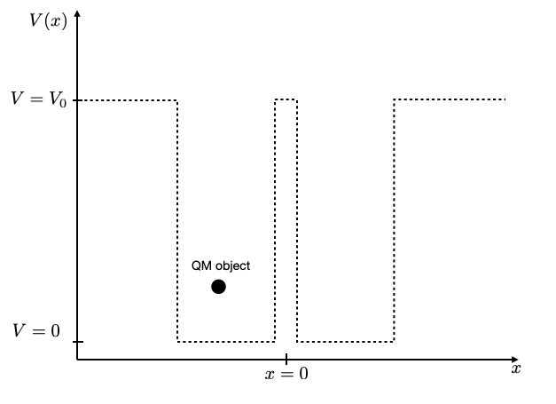
Here’s a starting point for exploring a double well: