Fourier Analysis

Fourier analysis, or the description of functions as a series of sine and cosine functions, serves as a powerful tool in both numerical data analysis and the solution of differential equations. In experimental physics, Fourier transforms find widespread applications. For instance, optical tweezers utilize frequency spectra to characterize positional fluctuations, while Lock-In detection employs Fourier analysis for specific frequency signals. Additionally, many optical phenomena can be understood through the lens of Fourier transforms.

Fourier analysis extends far beyond these examples, finding applications across numerous fields of physics and engineering. In this lecture, we will examine Fourier Series and Fourier transforms from a mathematical perspective. We will apply these concepts to analyze the frequency spectrum of oscillations in coupled pendula, and later revisit them when simulating the motion of a Gaussian wavepacket in quantum mechanics.

Fourier series

A Fourier series represents a periodic function \(f(t)\) with period \(2\pi\) or, more generally, any arbitrary interval \(T\) as a sum of sine and cosine functions:

\[ f(t)=\frac{A_{0}}{2}+\sum_{k=1}^{\infty}\left ( A_{k}\cos\left (\omega_k t\right) + B_{k}\sin\left (\omega_k t\right)\right ) \tag{1}\]

where \(\omega_k=\frac{2\pi k}{T}\). Here, \(T\) represents the period of the cosine and sine functions, with their amplitudes defined by the coefficients \(A_k\) and \(B_k\). The term \(A_0\) represents a constant offset added to the oscillating functions. Equation 1 expresses an arbitrary periodic function \(f(t)\) on an interval T as a sum of oscillating sine and cosine functions with discrete frequencies (\(\omega_k\)):

\[\begin{equation*} \omega_k= 0, \frac{2\pi}{T}, \frac{4\pi}{T}, \frac{6\pi}{T}, ... , \frac{n\pi}{T} \end{equation*}\]

and varying amplitudes. We can demonstrate that the cosine and sine functions in the sum (Equation 1) are orthogonal using the trigonometric identity:

\[\begin{equation} \sin(\omega_{i} t)\sin(\omega_{k}t )=\frac{1}{2}\lbrace\cos((\omega_{i}-\omega_{k})t)- \cos((\omega_{i}+\omega_{k})t\rbrace \end{equation}\]

This leads to the integral:

\[\begin{equation} \int\limits_{-\frac{T}{2}}^{+\frac{T}{2}} \sin(\omega_{i}t)\sin (\omega_k t) dt \end{equation}\]

which splits into two integrals over cosine functions with sum \((\omega_{1}+\omega_{2})\) and difference frequency \((\omega_{1}-\omega_{2})\). With \(\omega_k=k 2\pi/T\), \((k \in \mathbb{Z}^+ )\), this evaluates to:

\[\begin{equation} \int\limits_{-\frac{T}{2}}^{+\frac{T}{2}} \sin(\omega_{i}t)\sin (\omega_k t) dt =\begin{cases} 0 &\text{for } i\neq k, \\ T/2 &\text{for } i=k \end{cases} \end{equation}\]

A similar result holds for cosine functions:

\[\begin{equation} \int\limits_{-\frac{T}{2}}^{+\frac{T}{2}} \cos(\omega_{i}t)\cos (\omega_k t) dt =\begin{cases} 0 &\text{for } i\neq k, \\ T/2 &\text{for } i=k \end{cases} \end{equation}\]

The coefficients \(A_k\) and \(B_k\) are determined by projecting the function \(f(t)\) onto these basis functions:

\[\begin{align} \int\limits_{-\frac{T}{2}}^{+\frac{T}{2}} & \cos (\omega_k t) dt =\begin{cases} 0 &\text{for } k\neq0, \\ T &\text{for } k=0 \end{cases} \\ \int\limits_{-\frac{T}{2}}^{+\frac{T}{2}} & \sin(\omega_k t) dt=0 \text{ for all }k \end{align}\]

For the cosine coefficients:

\[\begin{equation}\label{A_k} A_k=\frac{2}{T}\int\limits_{-\frac{T}{2}}^{+\frac{T}{2}} f(t)\cos(\omega_k t) dt \text{ for } k \neq 0 \end{equation}\]

and the constant term:

\[\begin{equation} A_0= \frac{1}{T}\int\limits_{-\frac{T}{2}}^{+\frac{T}{2}} f(t) dt \end{equation}\]

Finally, for the sine coefficients:

\[\begin{equation}\label{B_k} B_k=\frac{2}{T}\int\limits_{-\frac{T}{2}}^{+\frac{T}{2}} f(t) \sin(\omega_k t) dt,\, \forall k \end{equation}\]

Physical interpretation of Fourier coefficients

The Fourier coefficients provide crucial physical insights about the original function:

• \(A_0\) represents the mean value or DC offset of the function over one period.
• \(A_k\) and \(B_k\) represent the strength (amplitude) of frequency components at \(\omega_k = \frac{2\pi k}{T}\).
• The larger the coefficient, the more that particular frequency contributes to the overall function.
• The power of a frequency component is proportional to \(A_k^2 + B_k^2\).
• The phase angle \(\phi_k = \tan^{-1}(-B_k/A_k)\) tells us the relative timing of each frequency component.

This decomposition allows us to understand complex signals as combinations of simpler oscillations. For instance, in a vibrating string, each coefficient corresponds to the amplitude of a particular harmonic. In an electrical circuit, these coefficients represent the amplitude of voltage or current at specific frequencies.

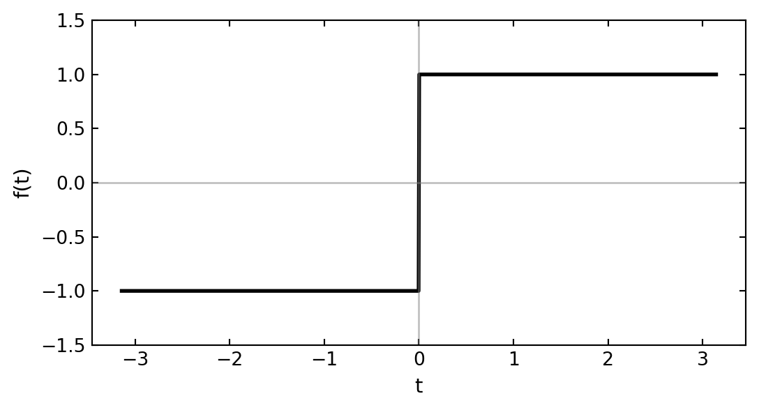
Example: Fourier series of a square wave

Let’s consider a concrete example: a square wave function with period \(T=2\pi\):

\[f(t) = \begin{cases} 1, & 0 < t < \pi \\ -1, & -\pi < t < 0 \end{cases}\]

Figure 1: Square Wave Function

This represents, for example, a signal that alternates between two voltage levels.

To find the Fourier coefficients, we have to determine the coefficients according to the integrals shown above. According to that, the DC component is:

\[A_0 = \frac{1}{2\pi}\int_{-\pi}^{\pi} f(t) dt = \frac{1}{2\pi}\left(\int_{-\pi}^{0} (-1) dt + \int_{0}^{\pi} 1 dt\right) = 0\]

Also, the coefficients for the cosine terms are:

\[A_k = \frac{1}{\pi}\int_{-\pi}^{\pi} f(t)\cos(kt) dt = \frac{1}{\pi}\left(\int_{-\pi}^{0} (-1)\cos(kt) dt + \int_{0}^{\pi} \cos(kt) dt\right) = 0 \, \text{for all } k\]

zero, as the cosine function is even and the square wave function is odd. Therefore, only the sine terms will contribute to the Fourier series.

\[B_k = \frac{1}{\pi}\int_{-\pi}^{\pi} f(t)\sin(kt) dt = \frac{1}{\pi}\left(\int_{-\pi}^{0} (-1)\sin(kt) dt + \int_{0}^{\pi} \sin(kt) dt\right)\]

Working through the integral, we find:

\[B_k = \frac{2}{\pi}\int_{0}^{\pi} \sin(kt) dt = \begin{cases} \frac{4}{k\pi}, & k \text{ odd} \\ 0, & k \text{ even} \end{cases}\]

Therefore, the Fourier series for our square wave is: \[f(t) = \frac{4}{\pi}\left(\sin(t) + \frac{1}{3}\sin(3t) + \frac{1}{5}\sin(5t) + \ldots\right) = \frac{4}{\pi}\sum_{n=0}^{\infty} \frac{1}{2n+1}\sin((2n+1)t)\]

Notice how adding more terms in the series makes the approximation closer to the true square wave. Also note that high-frequency components (larger k values) have smaller amplitudes, explaining why the approximation smoothes out the sharp transitions even with many terms.

Fourier transform

The Fourier transform extends the concept of Fourier series by representing arbitrary non-periodic functions \(f(t)\) through a continuous spectrum of complex functions \(\exp(i\omega t)\). Known as the continuous Fourier transform, this approach replaces the discrete frequency sum of sine and cosine functions found in Fourier series with an integral over complex exponential functions \(\exp(i\omega t)\) spanning continuous frequency values \(\omega\).

From Real to Complex Representation

Before diving into the Fourier transform, let’s clarify the transition from the real representation (sines and cosines) to the complex exponential notation. Using Euler’s formula:

\[e^{i\theta} = \cos(\theta) + i\sin(\theta)\]

We can rewrite our Fourier series from:

\[f(t)=\frac{A_{0}}{2}+\sum_{k=1}^{\infty}\left ( A_{k}\cos\left (\omega_k t\right) + B_{k}\sin\left (\omega_k t\right)\right )\]

to:

\[f(t)=\sum_{k=-\infty}^{\infty} c_k e^{i\omega_k t}\]

where \(c_k\) is a complex coefficient related to \(A_k\) and \(B_k\) by:

\[c_0 = \frac{A_0}{2}, \quad c_k = \frac{A_k - iB_k}{2}, \quad c_{-k} = \frac{A_k + iB_k}{2}\]

This complex representation often simplifies calculations and provides a more elegant mathematical formulation. The advantage becomes even more apparent when we move from discrete frequencies (Fourier series) to continuous frequencies (Fourier transform).

The Fourier transform of a function \(f(t)\) is defined as:

\[ F(\omega)=\int\limits_{-\infty}^{+\infty}f(t)e^{-i\omega t}dt \tag{2}\]

where \(F(\omega)\) represents the spectrum of frequencies present in \(f(t)\). The inverse Fourier transform recovers the original function \(f(t)\) from its frequency spectrum (Equation 2):

\[\begin{equation}\label{eq:inverse_FT} f(t)=\frac{1}{2\pi}\int\limits_{-\infty}^{+\infty}F(\omega)e^{+i\omega t}dt \end{equation}\]

The Fourier transform \(F(\omega)\) yields a complex number, encoding both phase and amplitude information of the oscillations. The phase of oscillation at frequency \(\omega\) is given by:

\[\begin{equation} \phi=\tan^{-1}\left(\frac{Im(F(\omega))}{Re(F(\omega))}\right) \end{equation}\]

while the amplitude at frequency \(\omega\) is:

\[\begin{equation} x_{0}^{\rm theo}=|F(\omega)| \end{equation}\]

Modern computing offers efficient algorithms for Fourier transformation, particularly the Fast Fourier Transform (FFT) implemented in libraries like NumPy. We’ll use these algorithms to identify oscillation patterns in our signals. Here’s an example of using NumPy’s FFT functions to compute the transform and generate the corresponding frequency axis:

f=np.fft.fft(alpha)

Frequency analysis of our coupled pendula

Let us now apply Fourier analysis to examine the data from our coupled pendula, which includes both normal modes and beat mode oscillations of the harmonic oscillator. Instead of using the numerical data from the simulation, we will use the analytical expressions for the normal modes and beat mode to demonstrate the Fourier analysis.

Analytical solution for coupled pendula

For two pendula with equal masses, coupled by a spring of constant \(k\), the equations of motion are:

\[\ddot{\theta}_1 + \omega_0^2\theta_1 + \kappa(\theta_1-\theta_2) = 0\] \[\ddot{\theta}_2 + \omega_0^2\theta_2 + \kappa(\theta_2-\theta_1) = 0\]

where \(\omega_0^2 = g/L\) is the natural frequency of a single pendulum and \(\kappa = k/m\) represents the coupling strength.

The normal mode frequencies are: \[\omega_1 = \omega_0 \quad \text{(in-phase mode)}\] \[\omega_2 = \sqrt{\omega_0^2 + 2\kappa} \quad \text{(out-of-phase mode)}\]

For the in-phase mode, both pendula move in sync: \[\theta_1(t) = \theta_2(t) = A\cos(\omega_1 t + \phi_1)\]

For the out-of-phase mode: \[\theta_1(t) = -\theta_2(t) = B\cos(\omega_2 t + \phi_2)\]

The beat mode results from the superposition of these normal modes: \[\theta_1(t) = A\cos(\omega_1 t) + B\cos(\omega_2 t)\] \[\theta_2(t) = A\cos(\omega_1 t) - B\cos(\omega_2 t)\]

When \(A = B\), this can be rewritten using trigonometric identities as: \[\theta_1(t) = 2A\cos\left(\frac{\omega_2-\omega_1}{2}t\right)\cos\left(\frac{\omega_2+\omega_1}{2}t\right)\] \[\theta_2(t) = 2A\sin\left(\frac{\omega_2-\omega_1}{2}t\right)\sin\left(\frac{\omega_2+\omega_1}{2}t\right)\]

This shows the characteristic beat pattern with a slow modulation (\(\frac{\omega_2-\omega_1}{2}\)) of a fast carrier frequency (\(\frac{\omega_2+\omega_1}{2}\)).

We can now perform the Fourier transform of our signals and visualize their frequency spectra. For the Fourier transform we will use the numpy.fft.fft() function.

NumPy FFT Functions

np.fft.fft(): This function computes the one-dimensional discrete Fourier transform of an input signal. It converts a time-domain signal into its frequency domain representation, revealing which frequency components are present in the signal and their respective amplitudes. The output is a complex array of the same size as the input, containing amplitude and phase information for each frequency component.

np.fft.fftfreq(): This complementary function generates the frequency values corresponding to the output of np.fft.fft(). It requires two arguments: the length of the signal and the sampling period (time step between consecutive points). The returned array contains both positive and negative frequencies, with zero frequency at the beginning. For physical interpretations, we typically focus on the positive frequencies only.

Together, these functions allow us to analyze oscillatory data by identifying its constituent frequencies - essential for understanding systems like coupled pendula, wave phenomena, or any periodic behavior.

Our analysis reveals that the beat mode represents a superposition of the system’s two normal modes. This demonstrates a fundamental principle: any possible state of a coupled oscillator system can be constructed from a superposition of its normal modes with specific amplitudes.

Interpreting Frequency Spectra in Physical Systems

The frequency spectra we’ve calculated provide deep insights into the physical behavior of the coupled pendula system:

1. Peak Locations: Each peak in the frequency spectrum corresponds to a characteristic frequency of the system. For our coupled pendula, these represent the natural frequencies of the normal modes.

2. Peak Heights: The amplitude of each peak indicates how strongly that particular frequency contributes to the overall motion. In our beat mode, we see roughly equal contributions from both normal mode frequencies, explaining the energy exchange between pendula.

3. Peak Width: The width of a frequency peak relates to damping in the system. Sharp, narrow peaks indicate weakly damped oscillations that persist for many cycles, while broader peaks suggest stronger damping.

4. Absence of Frequencies: The absence of certain frequencies is also informative. Our analysis shows only the two normal mode frequencies, confirming that our system behaves as expected for a coupled oscillator with two degrees of freedom.

When analyzing more complex systems, Fourier analysis becomes even more powerful. For instance, in quantum mechanics, the frequency spectrum of a wavefunction reveals its energy level structure; in structural engineering, it identifies resonant frequencies that could lead to catastrophic failure; and in signal processing, it helps distinguish meaningful signals from noise.

By understanding frequency domain representations alongside time domain behavior, we gain a complete picture of dynamical systems and their responses to various inputs.

Audio Signal Analysis with Fourier Transforms

In this exercise, you’ll analyze a mystery audio signal that contains multiple frequency components. The signal consists of a primary sound (like a voice) with its harmonics and some background noise.

1. Run the code to generate the mystery signal and view its frequency spectrum
2. From the FFT plot, identify:
   • The fundamental frequency of the primary sound
   • The harmonics present in the signal
   • The frequency of the background noise
3. Try modifying the signal components to see how the spectrum changes

Look for distinct peaks in the frequency spectrum. The tallest peak is likely the fundamental frequency, with smaller peaks at integer multiples (harmonics). A smaller isolated peak is likely the noise.

Solution