After having established that particles exhibit wave-like properties through phenomena such as electron diffraction, we need to develop a mathematical framework to describe matter waves. While a simple plane wave ansatz might seem like a natural starting point, we will see that it has limitations in describing localized particles. This leads us to the concept of wave packets and ultimately to a probabilistic interpretation of matter waves proposed by Max Born.
Plane waves
In order to properly describe the wave character of a particle with mass that is propagating along the direction we choose a similar ansatz as for electromagnetic light,
Even though we are still discussing properties of matter, the above equation has the shape of a wave function. Thus, one often refers to matter waves. In accord with the de Broglie wavelength and the analogous description of atomistic particles as waves, we can derive the kinetic energy as
and the momentum as
which allows us to reformulate the wave equation as
However, there is still an important distinction between photons of electromagnetic waves and corpuscles of matter waves. In the case of electromagnetic waves the phase velocity does not depend on the wave’s frequency. From the condition
it becomes evident that
and represents the vanishing dispersion of electromagnetic waves in vacuum . This relation does not hold true for matter waves. For a free particle (force-free motion in constant potential) we know
and
If we now make use of the definition of the phase velocity , it becomes evident that the dispersion relation gives:
Matter waves show dispersion and their phase velocity does depend on the wavevector and thus on the momentum of the particle. If the particle moves with the velocity , then
and the phase velocity of the matter waves corresponds to half the velocity of the particle. As a consequence, a matter wave and its phase velocity is not suited to describe the motion of particles without further considerations. Having in mind that a plane wave is distributed across the whole space, whereas a particle is somehow located, we provide remedy through the introduction of wave packets.
Wave packets
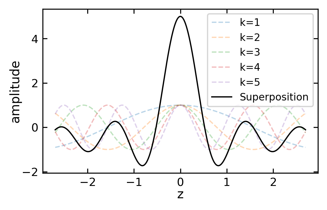
Unlike plane waves which extend infinitely in space, classical particles are localized. We can bridge this gap using wave packets (or wave trains) - superpositions of plane waves with similar frequencies and wavevectors:
Code
import numpy as npimport matplotlib.pyplot as plt# Set up the z-axisz = np.linspace(-2.7, 2.7, 1000)# Define 5 different wavenumbersk = [1, 2, 3, 4, 5]# Calculate individual waves and their superpositionwaves = []superposition = np.zeros_like(z)for ki in k: wave = np.cos(ki * z) waves.append(wave) superposition += wave# Plotplt.figure(figsize=get_size(10, 6))# Plot individual wavesfor i, wave inenumerate(waves): plt.plot(z, wave, '--', alpha=0.3, label=f'k={k[i]}')# Plot superpositionplt.plot(z, superposition, 'k-', linewidth=1, label='Superposition')plt.xlabel('z')plt.ylabel('amplitude')plt.legend()plt.show()
Superposition of five waves with different wavenumbers.
The wave packet has maximum amplitude at position , which propagates with the group velocity:
For a large number of waves with frequencies in and wavenumbers in , the sum becomes an integral:
The amplitude distribution and width determine the wave packet’s shape in momentum space.
Position of Maximum Amplitude
If we rewrite frequencies and wave vectors as deviations from central values:
The phase in the exponential then becomes . For constructive interference, the phases must be equal:
For neighboring waves , this means:
Subtracting the common terms from both sides gives:
This finally leads to the relation:
Therefore:
This gives the position of constructive interference, which is where the amplitude is maximum:
The derivative evaluated at is the group velocity, showing that the maximum of the wave packet moves with the group velocity.
Constant amplitude wave packets
If the width of the wavenumber interval is small compared to the wavenumber , we can expand in a Taylor series and neglect higher terms than the linear one resulting in
If further the amplitude does not change significantly on the interval (), we can replace through a constant . Now we get
with and . (Note: I had a typo in the integral equation on the blackboard. It was correct here.) The integration then results in
with
Code
# Parametersk0 =10.0# central wave numberomega0 =2.0# central frequencyC =1.0# amplitude constantt =0# time (starting at t=0)# Spatial gridz = np.linspace(-10, 10, 1000)# Create figure with two subplots side by sidefig, (ax1, ax2) = plt.subplots(1, 2, figsize=get_size(12, 6))# Plot for Delta_k = π/2Delta_k1 = np.pi/2u1 = omega0/k0 * t - zA1 =2* C * np.sinc(Delta_k1 * u1 / (2* np.pi))psi1 = A1 * np.exp(1j* (omega0 * t - k0 * z))ax1.plot(z, np.real(psi1), 'k-', label='Re(ψ)', alpha=0.7)ax1.plot(z, A1, 'r--', label='Envelope A(z,t)', linewidth=1)ax1.plot(z, -A1, 'r--', linewidth=1)ax1.set_xlabel('z')ax1.set_ylabel('ψ(z,t)')ax1.set_title(f'Wave Packet at t=0\nΔk = π/2')#ax1.legend()# Plot for Delta_k = πDelta_k2 = np.piu2 = omega0/k0 * t - zA2 =2* C * np.sinc(Delta_k2 * u2 / (2* np.pi))psi2 = A2 * np.exp(1j* (omega0 * t - k0 * z))ax2.plot(z, np.real(psi2), 'k-', label='Re(ψ)', alpha=0.7)ax2.plot(z, A2, 'r--', label='Envelope A(z,t)', linewidth=1)ax2.plot(z, -A2, 'r--', linewidth=1)ax2.set_xlabel('z')ax2.set_ylabel('ψ(z,t)')ax2.set_title(f'Wave Packet at t=0\nΔk = π')#ax2.legend()plt.tight_layout()plt.show()
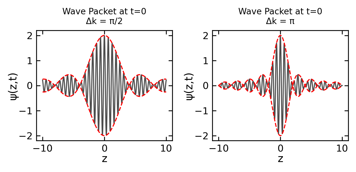
Constant amplitude wave packets for two different values of .
The function represents a plane wave whose amplitude exhibits a maximum at , and therefore . We call this function a wave packet. Its shape, namely height and distance to side lobes, does depend on the width of the interval and the distribution of the amplitude . The wave packet’s maximum propagates with the group velocity
along the direction. Moreover, we can make use of the relation
and derive for the group velocity
Thus, a wave packet is better suited than a plane wave for describing a particle on the microscopic scale, because characteristics of a wave packet can be interlinked with the according properties of a particle in the classical sense.
The wave packet’s group velocity corresponds to the particle’s velocity .
The wavevector of the packet’s center determines the momentum of the particle .
A wave packet is localized (in contrast to a plane wave) and the wave packet’s amplitude has maximum values only in a limited range . In the case we can calculate the width of the central maximum as distance between the roots . While this is sometimes incorrectly compared to the particle’s de Broglie wavelength , the actual width depends on the momentum spread and is not fundamentally limited by the wavelength.
Code
# ParametersN =1000# number of pointsx = np.linspace(-20, 20, N)dx = x[1] - x[0]k =2*np.pi*np.fft.fftfreq(N, dx) # momentum space gridk = np.fft.fftshift(k) # shift k-space gridtimes = [0, 2,4] # three different times# Create rectangular amplitude distribution in k-spacek0 =0.0# center wavevectordk =2.0# width in k-spacepsi_k = np.zeros(N, dtype=complex)mask = (k > k0-dk/2) & (k < k0+dk/2)psi_k[mask] =1.0# Function to calculate wavepacket at time tdef get_wavepacket(t):# Apply time evolution in k-space with dispersion# E = ℏ²k²/2m (using ℏ=m=1) E_k =0.5* k**2# quadratic dispersion relation psi_k_t = psi_k * np.exp(-1j* E_k * t)# Transform to position space psi_x = np.fft.ifftshift(np.fft.ifft(np.fft.ifftshift(psi_k_t)))return np.abs(psi_x)**2# Create three subplotsfig, (ax1, ax2, ax3) = plt.subplots(1, 3, figsize=get_size(12, 5))axes = [ax1, ax2, ax3]# Plot wavepacket at different timesfor ax, t inzip(axes, times): y = get_wavepacket(t) ax.plot(x, y/y.max(), 'b-') ax.set_xlim(-20, 20) ax.set_ylim(0, 1.2) ax.set_xlabel('position')if t ==0: ax.set_ylabel('prob. density') ax.set_title(f't = {t}')plt.tight_layout()plt.show()
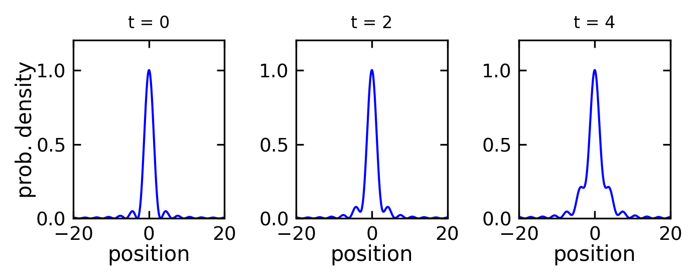
Constant amplitude wavepacket propagating in time and changing shape due to dispersion.
Gaussian wave packets
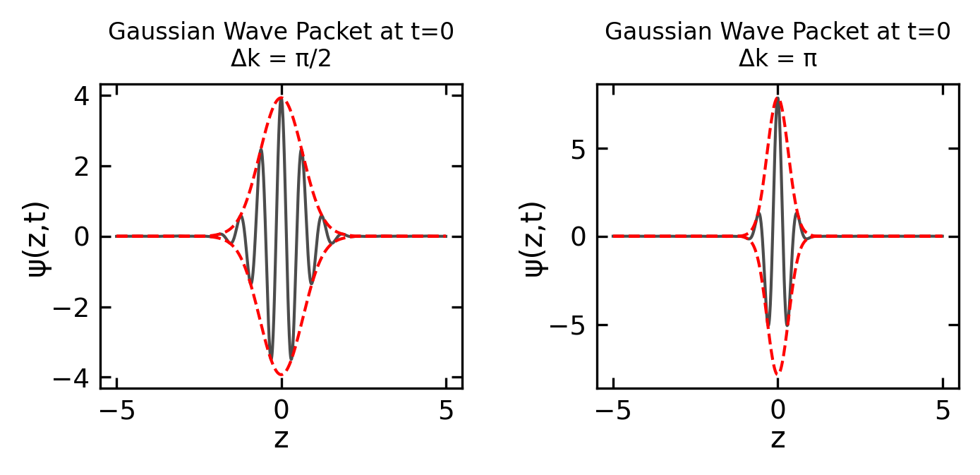
A Gaussian distribution for the amplitude provides an improved description of wave packets compared to constant amplitude:
The full wave function is then given by:
This wavefunction with the envelope is depicted below.
Code
# Parametersk0 =10.0# central wave numberomega0 =2.0# central frequencyC =1.0# amplitude constantt =0# time (starting at t=0)# Spatial gridz = np.linspace(-5, 5, 1000)# Create figure with two subplots side by sidefig, (ax1, ax2) = plt.subplots(1, 2, figsize=get_size(12, 6))# Function to create Gaussian wave packetdef gaussian_wavepacket(z, t, Delta_k): k = np.linspace(k0 -3*Delta_k, k0 +3*Delta_k, 1000) dk = k[1] - k[0]# Gaussian amplitude distribution C_k = C * np.exp(-(k - k0)**2/ (2* Delta_k**2))# Calculate wave packet through integration psi = np.zeros(len(z), dtype=complex)for i, ki inenumerate(k): psi += C_k[i] * np.exp(1j* (omega0 * t - ki * z)) * dkreturn psi# Plot for Delta_k = π/2Delta_k1 = np.pi/2psi1 = gaussian_wavepacket(z, t, Delta_k1)envelope1 = np.abs(psi1)ax1.plot(z, np.real(psi1), 'k-', label='Re(ψ)', alpha=0.7)ax1.plot(z, envelope1, 'r--', label='Envelope |ψ|', linewidth=1)ax1.plot(z, -envelope1, 'r--', linewidth=1)ax1.set_xlabel('z')ax1.set_ylabel('ψ(z,t)')ax1.set_title(f'Gaussian Wave Packet at t=0\nΔk = π/2')# Plot for Delta_k = πDelta_k2 = np.pipsi2 = gaussian_wavepacket(z, t, Delta_k2)envelope2 = np.abs(psi2)ax2.plot(z, np.real(psi2), 'k-', label='Re(ψ)', alpha=0.7)ax2.plot(z, envelope2, 'r--', label='Envelope |ψ|', linewidth=1)ax2.plot(z, -envelope2, 'r--', linewidth=1)ax2.set_xlabel('z')ax2.set_ylabel('ψ(z,t)')ax2.set_title(f'Gaussian Wave Packet at t=0\nΔk = π')plt.tight_layout()plt.show()
Gaussian wavpacket with different width in momentum space.
When integrated, the wave packet in position space has the envelope:
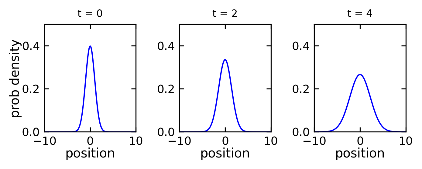
The time-dependent width evolves as:
where is the group velocity and is the initial width. The width spreads quadratically in time according to:
The spreading rate is governed by the initial width , Planck’s constant , and particle mass . Narrower packets and lighter particles spread more rapidly.
Code
# Parametershbar =1.0# reduced Planck's constantm =1.0# masssigma0 =1.0# initial widthk0 =2.0# initial wave numberx = np.linspace(-10, 10, 1000)times = [0, 2, 4] # three different times# Function to calculate wave packet at time tdef gaussian_packet(x, t):# Complex time-dependent width sigma_t = sigma0 * np.sqrt(1+ (1j*hbar*t)/(2*m*sigma0**2))# Normalization norm =1/np.sqrt(np.sqrt(2*np.pi)*sigma_t)# Gaussian envelope with phase psi = norm * np.exp(-(x**2)/(4*sigma_t**2)) * np.exp(1j*k0*x)return np.abs(psi)**2# Create three subplotsfig, (ax1, ax2, ax3) = plt.subplots(1, 3, figsize=get_size(12, 5))axes = [ax1, ax2, ax3]# Plot wavepacket at different timesfor ax, t inzip(axes, times): y = gaussian_packet(x, t) ax.plot(x, y, 'b-',) ax.set_xlim(-10, 10) ax.set_ylim(0, 0.5) ax.set_xlabel('position')if t ==0: ax.set_ylabel('prob density') ax.set_title(f't = {t}')plt.tight_layout()plt.show()
Gaussian wavepacket propagation. The width of the wavepacket changes in time due to the dispersion of massive particles.
Code
// Create plot containerviewof plot = {// Setup parametersconst width =600;const height =200;const margin = {top:20,right:20,bottom:40,left:60};// Physical constants (in natural units)const hbar =1;const m =1;const sigma0 =0.1;// initial widthconst k0 =50;// central wavevectorconst period =0.2;// time period for the loop// Create SVGconst svg = d3.create("svg").attr("width", width).attr("height", height);// Setup scalesconst x = d3.scaleLinear().domain([-2,15]).range([margin.left, width - margin.right]);const y = d3.scaleLinear().domain([0,3]).range([height - margin.bottom, margin.top]);// Add axes svg.append("g").attr("transform",`translate(0,${height - margin.bottom})`).call(d3.axisBottom(x).ticks(10)).append("text").attr("x", width/2).attr("y",35).attr("fill","black").text("Position"); svg.append("g").attr("transform",`translate(${margin.left},0)`).call(d3.axisLeft(y).ticks(5)).append("text").attr("transform","rotate(-90)").attr("x",-height/3).attr("y",-40).attr("fill","black").text("Probability Density");// Function to calculate wavepacket at time tfunctiongaussianPacket(x, t) {const sigma_t =Math.sqrt(sigma0**2+ (hbar*t/(2*m*sigma0))**2);const vg = hbar*k0/m;const x_shifted = x - (vg*t %20);// modulo for loopingreturnMath.exp(-x_shifted*x_shifted/(4*sigma_t*sigma_t))/(Math.sqrt(2*Math.PI*sigma_t*sigma_t)); }// Create line generatorconst line = d3.line().x(d =>x(d.x)).y(d =>y(d.y));// Animationlet t =0;const dt =0.001;functionupdate() {// Calculate wavepacketconst points = d3.range(-2,15,0.1).map(x => ({x: x,y:gaussianPacket(x, t % period) // use modulo for time looping }));// Update or create pathconst path = svg.selectAll("path.wavepacket").data([points]); path.enter().append("path").attr("class","wavepacket").merge(path).attr("fill","none").attr("stroke","blue").attr("stroke-width",2).attr("d", line);// Update time display svg.selectAll("text.time").data([`t = ${(t % period).toFixed(3)}`]).join("text").attr("class","time").attr("x", width -4*margin.right).attr("y", margin.top).text(d => d); t += dt;requestAnimationFrame(update);// removed conditional to make it loop }update();return svg.node();}
Despite these improvements, a wave packet still has limitations in modeling particles:
The wave function can take negative or complex values that don’t correspond to physical measurements
Wave packets spread over time due to dispersion, unlike classical particles
Waves can split into multiple parts, while elementary particles are indivisible
These limitations led Max Born to develop a statistical interpretation of matter waves.
The statistical interpretation of matter waves
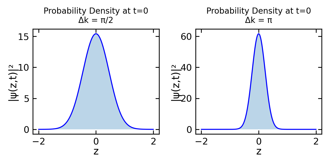
Max Born proposed a probabilistic interpretation of quantum mechanics where the wavefunction itself does not represent a physical quantity, but rather its absolute square gives the probability density for finding a particle at a particular position. For a particle described by a wavefunction , the probability of finding it within an infinitesimal interval at time is given by:
This interpretation arose from Born’s analysis of scattering problems, where he recognized that gives the probability of a particular scattering outcome. The wavefunction itself can take complex values, but its squared modulus is always real and non-negative, making it suitable as a probability density.
Since the particle must exist somewhere in space, the total probability of finding it anywhere must equal 1, leading to the normalization condition:
Code
# Parametersk0 =10.0# central wave numberomega0 =2.0# central frequencyC =1.0# amplitude constantt =0# time (starting at t=0)# Spatial gridz = np.linspace(-2, 2, 1000)# Create figure with two subplots side by sidefig, (ax1, ax2) = plt.subplots(1, 2, figsize=get_size(12, 6))# Function to create Gaussian wave packetdef gaussian_wavepacket(z, t, Delta_k): k = np.linspace(k0 -3*Delta_k, k0 +3*Delta_k, 1000) dk = k[1] - k[0]# Gaussian amplitude distribution C_k = C * np.exp(-(k - k0)**2/ (2* Delta_k**2))# Calculate wave packet through integration psi = np.zeros(len(z), dtype=complex)for i, ki inenumerate(k): psi += C_k[i] * np.exp(1j* (omega0 * t - ki * z)) * dkreturn psi# Plot for Delta_k = π/2Delta_k1 = np.pi/2psi1 = gaussian_wavepacket(z, t, Delta_k1)prob_density1 = np.abs(psi1)**2ax1.plot(z, prob_density1, 'b-', label='|ψ|²')ax1.fill_between(z, prob_density1, alpha=0.3)ax1.set_xlabel('z')ax1.set_ylabel('|ψ(z,t)|²')ax1.set_title(f'Probability Density at t=0\nΔk = π/2')# Plot for Delta_k = πDelta_k2 = np.pipsi2 = gaussian_wavepacket(z, t, Delta_k2)prob_density2 = np.abs(psi2)**2ax2.plot(z, prob_density2, 'b-', label='|ψ|²')ax2.fill_between(z, prob_density2, alpha=0.3)ax2.set_xlabel('z')ax2.set_ylabel('|ψ(z,t)|²')ax2.set_title(f'Probability Density at t=0\nΔk = π')plt.tight_layout()plt.show()
The squared wave packet with a Gaussian amplitude distribution (black line) and probability density (area under the curve, shaded gray).
In the case the particle propagates within a three-dimensional space, we can assign a three-dimensional wave packet to this particle. As discussed above, the particle has to be located somewhere in space and as a consequence the probability to find it within the whole space is and we can state the normalization condition
Thus, we can conclude:
Every particle can be represented through a matter wave being determined through the wave function .
The quantity with its normalization represents the probability to find the particle within the volume element at the particular time .
The probability to find the particle is biggest at the center of the wave packet.
The center of the wave packet propagates with the group velocity which is identical to the classical particle velocity .
The probability to find the particle within an infinite volume is not . This means one cannot locate the particle in a single spot . The particle’s location is smeared which corresponds to the distribution of the wave packet and obeys an uncertainty.
Relation to measurement
The probabilistic interpretation of the wave function has profound implications for the measurement process in quantum mechanics. When we perform a measurement on a quantum system:
The act of measurement causes the wave function to “collapse” from its spread-out state to a localized state
Before measurement, the particle exists in a superposition described by the wave function
The measurement outcome will be random, but governed by the probability distribution
After measurement, the wave function collapses to a new state centered on the measured position
Subsequent measurements will find the particle near this new position until the wave packet spreads out again due to time evolution
This measurement-induced collapse of the wave function is a key feature that distinguishes quantum mechanics from classical physics. It represents the transition from quantum probabilities to definite classical outcomes. The spreading of wave packets between measurements represents the return to quantum uncertainty.
The question of whether wavefunction collapse occurs during non-destructive measurements is actually still debated in quantum mechanics. While traditional Copenhagen interpretation suggests collapse occurs with any measurement, modern perspectives like quantum decoherence offer alternative views.
Non-destructive measurements (also called QND - Quantum Non-Demolition measurements) can preserve the quantum state while still extracting some information. However, they still cause some level of interaction/entanglement between the system and measuring apparatus.
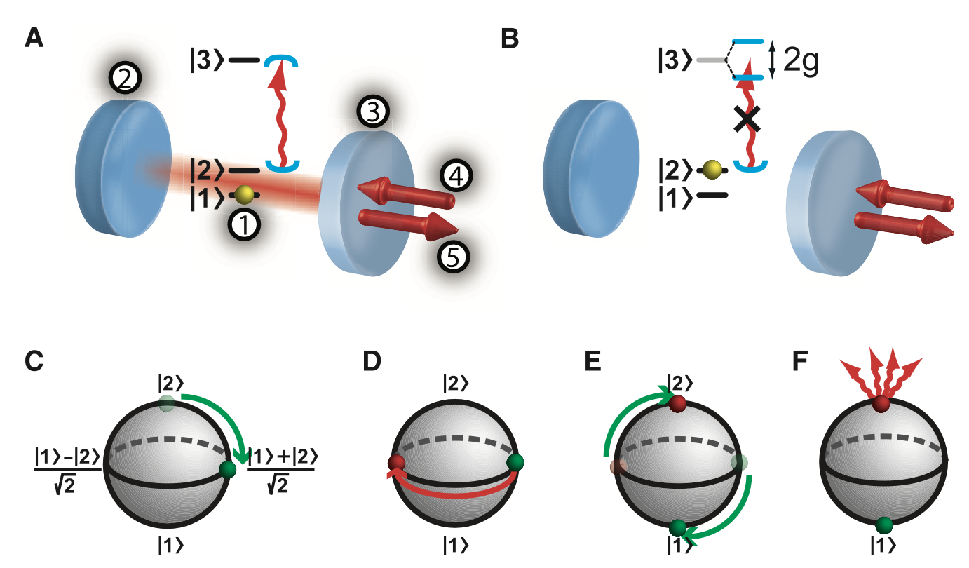
The authors developed a specific measurement scheme, that allows to detect the presence of a single photon without destroying it.
Figure 1— Nondestructive photon detection. (A and B) Sketch of the setup and atomic level scheme. A single atom, (1), is trapped in an optical cavity that consists of a high-reflector, (2), and a coupling mirror, (3). A resonant photon is impinging on, (4), and reflected off, (5), the cavity. (A) If the atom is in state , the photon (red wavy arrow) enters the cavity (blue semicircles) before being reflected. In this process, the combined atom-photon state acquires a phase shift of . (B) If the atom is in , the strong coupling on the transition leads to a normal-mode splitting of , so that the photon cannot enter the cavity and is directly reflected without a phase shift. (C to F) Procedure to measure whether a photon has been reflected. (C) The atomic state, visualized on the Bloch sphere, is prepared in the superposition state . ( D ) If a photon impinges, the atomic state is flipped to . (E) The atomic state is rotated by . (F) Fluorescence detection is used to discriminate between the states and . Taken from Nondestructive Detection of an Optical Photon