Multiple Wave Interference

So far we looked at the interference of two waves, which was a simplification as I mentioned already earlier. Commonly there will be a multitude of partial waves contribute to the oberved intereference. This is what we would like to have a look at now. We will do that in a quite general fashion, as the resulting formulas will appear several times again for different problems.

Nevertheless we will make a difference between

• multiwave interference of waves with the constant amplitude
• multiwave interference of waves with decreasing amplitude

Especially the latter is often occuring, if we have multiple reflections and each reflection is only a fraction of the incident amplitude.

Multiple Wave Interference with Constant Amplitude

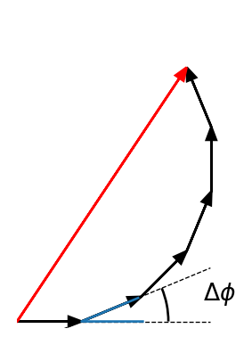
In the case of constant amplitude (for example realized by a grating, which we talk about later), the total wave amplitude is given according to the picture below by

$$U=U_1+U_2+U_1+U_3+\dots +U_M$$

where we sum the amplitude over $M$ partial waves. Between the neighboring waves (e.g. $U_1$ and $U_2$), we will assume a phase difference (because of a path length difference for example), which we denote as $\mathrm{\Delta }\varphi$.

The amplitude of the p-th wave is then given by

$$U_p=\sqrt{I_0}{e}^{i(p-1)\mathrm{\Delta }\varphi }$$

with the index $p$ being an interger $p=1,2,\dots ,M$, $h=e^{i\mathrm{\Delta }\varphi }$ and $\sqrt{I_0}$ as the amplitude of each individual wave. The total amplitude $U$ can be then expressed as

$$U=\sqrt{I_0}(1+h+h^2+\dots +h^{M-1})$$

which is a geometric sum. We can apply the sum formula for geometric sums to obtain

$$U=\sqrt{I_0}\frac{1-h^M}{1-h}=\sqrt{I_0}\frac{1-e^{iM\mathrm{\Delta }\varphi }}{1-e^{i\mathrm{\Delta }\varphi }}$$

We now have to calculate the intensity of the total amplitude

$$I=|U{|}^2=I_0{\left|\frac{e^{-iM\mathrm{\Delta }\varphi /2}-e^{iM\mathrm{\Delta }\varphi /2}}{e^{-i\mathrm{\Delta }\varphi /2}-e^{i\mathrm{\Delta }\varphi /2}}\right|}^2$$

which we can further simplify to give

$$I=I_0\frac{{\sin }^2(M\mathrm{\Delta }\varphi /2)}{{\sin }^2(\mathrm{\Delta }\varphi /2)}$$

# Parameters
M = 6  # number of phasors
phi = np.pi/8  # example phase difference between successive phasors

def plot_angle(ax, pos, angle, length=0.95, acol="C0", **kwargs):
    vec2 = np.array([np.cos(np.deg2rad(angle)), np.sin(np.deg2rad(angle))])
    xy = np.c_[[length, 0], [0, 0], vec2*length].T + np.array(pos)
    ax.plot(*xy.T, color=acol)
    return AngleAnnotation(pos, xy[0], xy[2], ax=ax, **kwargs)

# Calculate phasor positions
def calculate_phasors(phi, M):
    # Initialize arrays for arrow start and end points
    x_start = np.zeros(M)
    y_start = np.zeros(M)
    x_end = np.zeros(M)
    y_end = np.zeros(M)

    # Running sum of phasors
    x_sum = 0
    y_sum = 0

    for i in range(M):
        # Current phasor
        x = np.cos(i * phi)
        y = np.sin(i * phi)

        # Store start point (end of previous phasor)
        x_start[i] = x_sum
        y_start[i] = y_sum

        # Add current phasor
        x_sum += x
        y_sum += y

        # Store end point
        x_end[i] = x_sum
        y_end[i] = y_sum

    return x_start, y_start, x_end, y_end

x_start, y_start, x_end, y_end = calculate_phasors(phi, M)

plt.figure(figsize=get_size(6, 6))
ax = plt.gca()

for i in range(M):
    plt.arrow(x_start[i], y_start[i],
             x_end[i]-x_start[i], y_end[i]-y_start[i],
             head_width=0.15, head_length=0.2, fc='k', ec='k',
             length_includes_head=True,
             label=f'E{i+1}' if i == 0 else "")

plt.arrow(0, 0, x_end[-1], y_end[-1],
         head_width=0.15, head_length=0.2, fc='r', ec='r',
         length_includes_head=True, label='Resultant')

ax.set_aspect('equal')
xx = np.linspace(-1, 3, 100)
ax.plot(xx,(xx-1)*np.tan(phi),'k--',lw=0.5)
ax.plot([1,3],[0,0],'k--',lw=0.5)
kw = dict(size=195, unit="points", text=r"$\Delta \phi$")
plot_angle(ax, (1.0, 0), phi*180/np.pi, textposition="inside", **kw)
plt.axis('off')
max_range = max(abs(x_end[-1]), abs(y_end[-1])) * 1.2
plt.xlim(-0, max_range/1.5)
plt.ylim(-0.1, max_range/1.)

plt.show()
# Parameters
M = 6
phi = np.linspace(-4*np.pi, 4*np.pi, 10000)  # increased resolution
I0 = 1

def multiple_beam_pattern(phi, M):
    numerator = np.sin(M * phi/2)**2
    denominator = np.sin(phi/2)**2
    I = np.where(denominator != 0, numerator/denominator, M**2)
    return I

I = I0 * multiple_beam_pattern(phi, M)

first_min = 2*np.pi/M  # theoretical value

def find_nearest(array, value):
    array = np.asarray(array)
    idx = (np.abs(array - value)).argmin()
    return array[idx], idx

half_max = M**2/2

phi_positive = phi[phi >= 0]  # only positive values
I_positive = I[phi >= 0]
_, idx_half = find_nearest(I_positive, half_max)
half_width = phi_positive[idx_half]

# Create plot
plt.figure(figsize=get_size(10, 6))
plt.plot(phi/np.pi, I, 'b-', label=f'M={M}')

#plt.plot(first_min/np.pi, multiple_beam_pattern(first_min, M), 'ro')
#plt.annotate(f'First minimum\nφ = 2π/M = {first_min/np.pi:.2f}π',

plt.axvline(x=first_min/np.pi, color='r', linestyle='--', label=f'φ = 2π/M = {first_min/np.pi:.2f}π')

#plt.plot(half_width/np.pi, half_max, 'go')

plt.xlabel(r'phase $\Delta \phi/\pi$')
plt.ylabel('intensity I/I₀')
plt.title(f'Multiple Beam Interference Pattern (M={M})')
plt.ylim(0, M**2 + 15)
plt.legend()
plt.show()

Multiple wave interference of $M=6$ waves with a phase difference of $\varphi =\pi /8$. The black arrows represent the individual waves, the red arrow the sum of all waves.

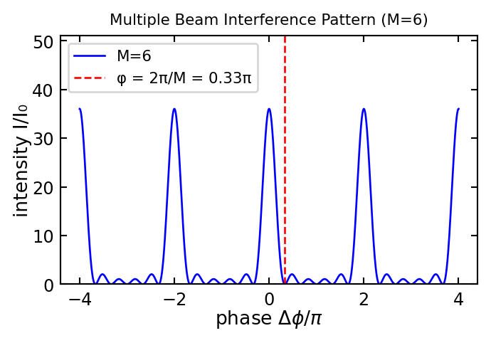
Figure 1— Multiple beam interference pattern for M=6 beams. The intensity distribution is shown as a function of the phase shift $\varphi$. The first minimum is at $\varphi =2\pi /M$. The intensity distribution is symmetric around $\varphi =0$.

The result is therefore an oscillating function. The numerator ${\sin }^2(M\mathrm{\Delta }\varphi /2)$ shows and oscillation frequency, which is by a factor of $M$ higher than the one in the denominator ${\sin }^2(\mathrm{\Delta }\varphi /2)$. Therefore the intensity pattern is oscillating rapidly and creating a first minimum at

$$\mathrm{\Delta }\varphi =\frac{2\pi }{M}$$

This is an important result, since it shows that the number of sources $M$ determines the position of the first minimum and the interference peak gets narrower with increasing $M$. Since the phase difference $\mathrm{\Delta }\varphi$ between neighboring sources is the same as for the double slit experiment, i.e. $\mathrm{\Delta }\varphi =2\pi d/\lambda \sin (\theta )$, we can also determine the angular position of the first minimum. This is given by

$$\sin ({\theta }_{\text{min}})=\frac{1}{M}\frac{\lambda }{d}$$

This again has the common feature that it scales as $\lambda /d$. A special situation occurs, whenever the numerator and the denominator become zero. This will happen whenever

$$\mathrm{\Delta }\varphi =m2\pi$$

where $m$ is an integer and denotes the interference order, i.e. the number of wavelength that neighboring partial waves have as path length difference. In this case, the intensity distributiion will give us

$$I=I_0\frac{0}{0}$$

and we have to determine the limit with the help of l’Hospitals rule. The outcome of this calculation is, that

$$I(\mathrm{\Delta }\varphi =m2\mathrm{\Delta }\pi )=M^2{I}_0$$

which can be also realized when using the small angle approximation for the sine functions.

Wavevector Representation

We would like to introduce a different representation of the multiple wave interference of the grating, which is quite insightful. The first order ($m=1$) constructive interference condition is given by

$$\frac{1}{\lambda }\sin \theta =\frac{1}{d}$$

which also means that

$$\frac{2\pi }{\lambda }\sin \theta =\frac{2\pi }{d}$$

This can be written as

$$k\sin \theta =K$$

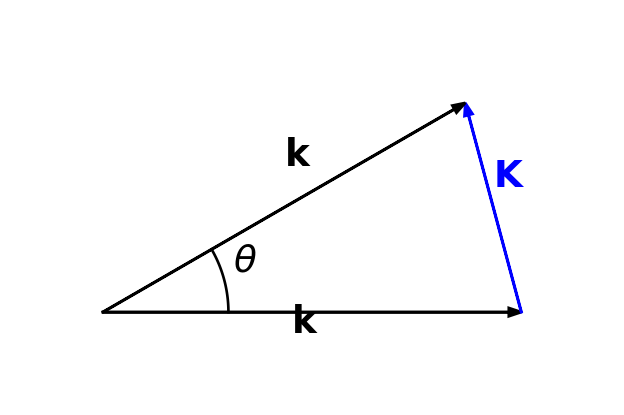
where $k$ is the magnitude of the wavevector of the light and $K$ is the wavevector magnitude that corresponds to the grating period $d$. As the magnitude of the wavevector of the light is conserved, the wavevectors of the incident light and the light traveling along the direction of the first interence peak form the sides of an equilateral triangle. This is shown in the following figure.

import numpy as np
import matplotlib.pyplot as plt


k = 1  # Magnitude of k₁ and k₂

origin = np.array([0, 0])

k1 = np.array([k, 0])

theta_deg = 30  # θ = 30 degrees
theta_rad = np.deg2rad(theta_deg)

k2 = k * np.array([np.cos(theta_rad), np.sin(theta_rad)])

K = k2 - k1

point_O = origin
point_A = point_O + k1
point_B = point_O + k2


plt.figure(figsize=get_size(10, 10))
ax = plt.gca()

# Plot vector k₁
ax.arrow(point_O[0], point_O[1], k1[0], k1[1],
         head_width=0.02, head_length=0.03, fc='k', ec='k', length_includes_head=True)


ax.arrow(point_A[0], point_A[1], K[0], K[1],
         head_width=0.02, head_length=0.03, fc='b', ec='b', length_includes_head=True)

ax.arrow(point_O[0], point_O[1], k2[0], k2[1],
         head_width=0.02, head_length=0.03, fc='k', ec='k', length_includes_head=True)

# Label vectors
ax.text(k1[0]/2 - 0.05, k1[1]/2 - 0.05, r'$\mathbf{k}$', fontsize=14, color='k')
ax.text(point_A[0] + K[0]/2 , point_A[1] + K[1]/2 + 0.05, r'$\mathbf{K}$', fontsize=14, color='b')
ax.text(k2[0]/2 + 0.0, k2[1]/2+0.1, r'$\mathbf{k}$', fontsize=14, color='k')

# Indicate angle θ between k₁ and k₂ at the origin
arc_radius = 0.3  # Radius of the arc representing θ
angle_range = np.linspace(0, theta_rad, 100)
arc_x = arc_radius * np.cos(angle_range)
arc_y = arc_radius * np.sin(angle_range)
ax.plot(arc_x, arc_y, color='k')

ax.text(arc_radius * np.cos(theta_rad / 2) + 0.02,
        arc_radius * np.sin(theta_rad / 2) + 0.02,
        r'$\theta$', fontsize=14)

# Set equal aspect ratio
ax.set_aspect('equal', adjustable='box')

all_x = [point_O[0], point_A[0], point_B[0]]
all_y = [point_O[1], point_A[1], point_B[1]]
margin = 0.2
ax.set_xlim(min(all_x) - margin, max(all_x) + margin)
ax.set_ylim(min(all_y) - margin, max(all_y) + margin)
plt.axis('off')

# Display the plot
plt.show()

Wavevector summation for the diffraction grating. The wavevector of the incident light $k$ and the wavevector of the light traveling along the direction of the first interference peak $K$ form an equilateral triangle.

This means that the diffraction grating is providing a wavevector $K$ to alter the direction of the incident light. This is again a common feature reappearing in many situations as for example in the X-ray diffraction of crystals.

Multiple Wave Interference with Decreasing Amplitude

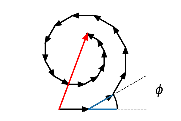
We will turn our attention now to a slight modification of the previous multiwave interference. We will introduce a decreasing amplitude of the individual waves. The first wave shall have an amplitude $U_1=\sqrt{I_0}$. The next wave, however, will not only be phase shifted but also have a smaller amplitude.

$$U_2=h{U}_1$$

where $h=r{e}^{i\varphi }$ with $|h|=r<1$. $r$ can be regarded as a reflection coefficient, which deminishes the amplitude of the incident wave. According to that the intensity is reduced by

$$I_2=|U_2{|}^2=|h{U}_1{|}^2=r^2{I}_1$$

The intensity of the incident wave is multiplied by a factor $r^2$, while the amplitude is multiplied by $r$. Note that the phase factor $e^{i\mathrm{\Delta }\varphi }$ is removed when taking the square of this complex number.

Intensity at Boundaries

The amplitude of the reflected wave is diminished by a factor $r\le 1$, which is called the reflection coefficient. The intensity is diminished by a factor $R=|r{|}^2\le 1$, which is the reflectance.

In the absence of absorption, reflectance $R$ and transmittance $T$ add to one due to energy conservation.

$$R+T=1$$

Consequently, the third wave would be now $U_3=h{U}_2=h^2{U}_1$. The total amplitude is thus

$$U=U_1+U_2+U_3+\dots +U_M=\sqrt{I_0}(1+h+h^2+\dots )$$

M = 18  # number of phasors
phi = np.pi/6  # example phase difference between successive phasors
r = 0.95  # reduction factor for each subsequent phasor

def plot_angle(ax, pos, angle, length=0.95, acol="C0", **kwargs):
    vec2 = np.array([np.cos(np.deg2rad(angle)), np.sin(np.deg2rad(angle))])
    xy = np.c_[[length, 0], [0, 0], vec2*length].T + np.array(pos)
    ax.plot(*xy.T, color=acol)
    return AngleAnnotation(pos, xy[0], xy[2], ax=ax, **kwargs)

def calculate_phasors(phi, M, r):
    x_start = np.zeros(M)
    y_start = np.zeros(M)
    x_end = np.zeros(M)
    y_end = np.zeros(M)

    x_sum = 0
    y_sum = 0

    for i in range(M):
        amplitude = r**i  # exponential decrease
        x = amplitude * np.cos(i * phi)
        y = amplitude * np.sin(i * phi)

        x_start[i] = x_sum
        y_start[i] = y_sum

        x_sum += x
        y_sum += y

        x_end[i] = x_sum
        y_end[i] = y_sum

    return x_start, y_start, x_end, y_end

x_start, y_start, x_end, y_end = calculate_phasors(phi, M, r)

plt.figure(figsize=get_size(6, 6),dpi=150)
ax = plt.gca()

for i in range(M):
    plt.arrow(x_start[i], y_start[i],
             x_end[i]-x_start[i], y_end[i]-y_start[i],
             head_width=0.15, head_length=0.2,
             fc='k', ec='k',
             length_includes_head=True,
             label=f'E{i+1}' if i == 0 else "")

plt.arrow(0, 0, x_end[-1], y_end[-1],
         head_width=0.15, head_length=0.2, fc='r', ec='r',
         length_includes_head=True, label='Resultant')

ax.set_aspect('equal')
xx = np.linspace(-1, 3, 100)
ax.plot(xx,(xx-1)*np.tan(phi),'k--',lw=0.5)
ax.plot([1,3],[0,0],'k--',lw=0.5)
kw = dict(size=195, unit="points", text=r"$\phi$")
plot_angle(ax, (1.0, 0), phi*180/np.pi, textposition="inside", **kw)
plt.axis('off')
max_range = max(abs(x_end[-1]), abs(y_end[-1])) * 1.2
plt.xlim(-max_range/1.8, max_range/0.8)
plt.ylim(-0.1, max_range/0.9)

plt.show()
import numpy as np
import matplotlib.pyplot as plt

# Create phase array from -2π to 2π
phi = np.linspace(-2*np.pi, 2*np.pi, 1000)

def calculate_intensity(phi, F):
    return 1/(1 + 4*(F/np.pi)**2 * np.sin(phi/2)**2)

plt.figure(figsize=get_size(10, 6))

finesse_values = [1, 4, 20]
styles = ['-', '--', ':']

for F, style in zip(finesse_values, styles):
    I = calculate_intensity(phi, F)
    plt.plot(phi/np.pi, I, style, label=f'$\\mathcal{{F}}={F}$')

plt.xlabel('Phase $\\phi/\\pi$')
plt.ylabel('$I/I_{\\mathrm{max}}$')
plt.grid(True, alpha=0.3)
plt.legend()
plt.ylim(0, 1.1)

plt.show()

Phase construction of a multiwave intereference with M waves with decreasing amplitude due to a reflection coefficient $r=0.95$.

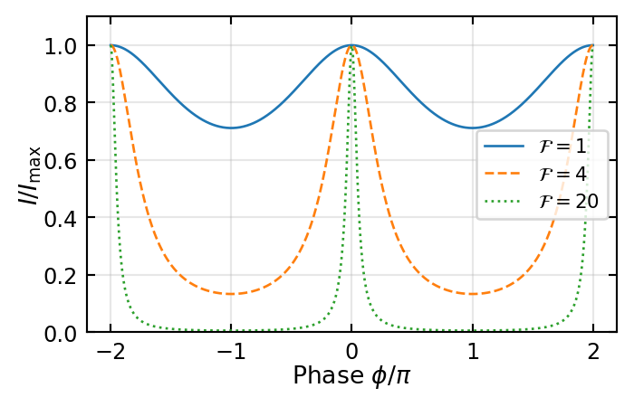
Multiple wave interference with decreasing amplitude. The graph shows the intensity distribution over the phase angle $\varphi$ for different values of the Finesse $\mathcal{F}$.

This yields again

$$U=\sqrt{I_0}\frac{(1-h^M)}{1-h}=\frac{\sqrt{I_0}}{1-r{e}^{i\mathrm{\Delta }\varphi }}$$

Calculating the intensity of the waves is giving

$$I=|U{|}^2=\frac{I_0}{|1-r{e}^{i\mathrm{\Delta }\varphi }{|}^2}=\frac{I_0}{(1-r{)}^2+4r{\sin }^2(\mathrm{\Delta }\varphi /2)}$$

which is also known as the Airy function. This function can be further simplified by the following abbrevations

$$I_{\mathrm{m}\mathrm{a}\mathrm{x}}=\frac{I_0}{(1-r{)}^2}$$

and

$$\mathcal{F}=\frac{\pi \sqrt{r}}{1-r}$$

where the latter is called the Finesse. With those abbrevations, we obtain

$$I=\frac{I_{\mathrm{m}\mathrm{a}\mathrm{x}}}{1+4{\left(\frac{\mathcal{F}}{\pi }\right)}^2{\sin }^2(\mathrm{\Delta }\varphi /2)}$$

for the interference of multiple waves with decreasing amplitude.

This intensity distribution has a different shape than the one we obtained for multiple waves with the same amplitude.

We clearly observe that with increasing Finesse the intensity maxima, which occur at multiples fo $\pi$ get much narrower. In addition the regions between the maxima show better contrast and fopr higher Finesse we get complete destructive interference.