Principles of Nonlinear Optics
In conventional (linear) optics, the response of a material to an applied electric field is linearly proportional to the field strength. This can be understood through a simple mechanical picture where electrons in atoms are treated as if they’re bound to the nucleus by springs with linear restoring forces (following Hooke’s law). When an electric field from light interacts with these electrons, they oscillate around their equilibrium positions. In the linear regime, this oscillation occurs precisely at the frequency of the incident light, and the displacement is directly proportional to the field strength.
However, when light becomes intense enough, typically from laser sources, this simple picture breaks down. The “springs” binding the electrons become anharmonic, with restoring forces that include nonlinear terms in the displacement. As a result, electrons no longer oscillate in simple harmonic motion but follow more complex trajectories that contain frequency components beyond the driving frequency. This nonlinear motion of the charges produces electromagnetic radiation at new frequencies not present in the incident light, forming the foundation of nonlinear optics, a field with numerous applications in modern technology and fundamental research.
Linear vs. Nonlinear Optical Response
The Linear Regime
In the linear regime, the polarization \(\mathbf{P}\) of a material is directly proportional to the applied electric field \(\mathbf{E}\):
\[\mathbf{P} = \varepsilon_0 \chi^{(1)} \mathbf{E}\]
where \(\varepsilon_0\) is the permittivity of free space and \(\chi^{(1)}\) is the linear susceptibility tensor.
This polarization field contributes to Maxwell’s equations, specifically through the electric displacement field \(\mathbf{D} = \varepsilon_0 \mathbf{E} + \mathbf{P}\). Starting with Maxwell’s equations in a source-free dielectric medium:
\[\nabla \times \mathbf{E} = -\frac{\partial \mathbf{B}}{\partial t}\] \[\nabla \times \mathbf{H} = \frac{\partial \mathbf{D}}{\partial t}\]
We can derive the wave equation:
\[\nabla^2 \mathbf{E} - \mu_0 \frac{\partial^2 \mathbf{D}}{\partial t^2} = 0\]
Substituting the linear polarization relation, we get:
\[\nabla^2 \mathbf{E} - \mu_0 \frac{\partial^2}{\partial t^2}[\varepsilon_0 \mathbf{E} + \varepsilon_0 \chi^{(1)} \mathbf{E}] = 0\]
\[\nabla^2 \mathbf{E} - \mu_0 \varepsilon_0 (1 + \chi^{(1)}) \frac{\partial^2 \mathbf{E}}{\partial t^2} = 0\]
Defining the relative permittivity \(\varepsilon_r = 1 + \chi^{(1)}\) and refractive index \(n = \sqrt{\varepsilon_r}\), and using \(c = \frac{1}{\sqrt{\mu_0 \varepsilon_0}}\) for the speed of light in vacuum, the wave equation becomes:
\[\nabla^2 \mathbf{E} - \frac{n^2}{c^2} \frac{\partial^2 \mathbf{E}}{\partial t^2} = 0\]
This transformed wave equation shows that the phase velocity in the medium is \(v_p = \frac{c}{n}\), demonstrating how the material’s linear response modifies the propagation of light through the medium.
The Nonlinear Regime
When the applied field becomes strong, we need to express the polarization as a power series:
\[\mathbf{P} = \varepsilon_0 [\chi^{(1)} \mathbf{E} + \chi^{(2)} \mathbf{E}^2 + \chi^{(3)} \mathbf{E}^3 + ...]\]
where \(\chi^{(2)}\) and \(\chi^{(3)}\) are the second-order and third-order nonlinear susceptibility tensors, respectively.
To understand how this nonlinear polarization affects light propagation, we can separate the polarization into linear and nonlinear parts:
\[\mathbf{P} = \mathbf{P}^{(1)} + \mathbf{P}^{NL}\]
where \(\mathbf{P}^{(1)} = \varepsilon_0 \chi^{(1)} \mathbf{E}\) is the linear polarization and \(\mathbf{P}^{NL} = \varepsilon_0 [\chi^{(2)} \mathbf{E}^2 + \chi^{(3)} \mathbf{E}^3 + ...]\) is the nonlinear polarization.
Substituting this into the wave equation derived earlier, we get:
\[\nabla^2 \mathbf{E} - \mu_0 \frac{\partial^2}{\partial t^2}[\varepsilon_0 \mathbf{E} + \mathbf{P}^{(1)} + \mathbf{P}^{NL}] = 0\]
Rearranging terms and using the definition of the linear refractive index:
\[\nabla^2 \mathbf{E} - \frac{n^2}{c^2} \frac{\partial^2 \mathbf{E}}{\partial t^2} = \mu_0 \frac{\partial^2 \mathbf{P}^{NL}}{\partial t^2}\]
This reformulation of the wave equation reveals a critical insight: the nonlinear polarization term acts as a source term in the wave equation. The left side describes wave propagation in a linear medium, while the right side represents a driving term arising from nonlinear optical processes.
The Born approximation provides a useful framework for analyzing this equation. This approximation assumes that the nonlinear effects are much weaker than the linear response, allowing us to treat the nonlinear polarization as a perturbation. Under this approximation, we first solve for the electric field considering only linear effects, then use this solution to calculate the nonlinear polarization, which in turn acts as a source for new field components.
Physically, this means that the nonlinear medium not only modifies the incident light but actually generates new electromagnetic radiation at different frequencies. For example, when the nonlinear polarization contains a term oscillating at frequency \(2\omega\) (as in second-harmonic generation), it acts as a source that radiates an electromagnetic wave at this new frequency. This perspective elegantly explains how nonlinear optical processes can create light with frequencies not present in the original input fields.
Second-Order Nonlinear Processes
Second-order nonlinear effects occur only in materials without inversion symmetry. This fundamental restriction arises from symmetry considerations: in a material with inversion symmetry, if we apply an electric field \(\mathbf{E}\), the induced polarization \(\mathbf{P}\) must change sign if \(\mathbf{E}\) changes sign. Mathematically, if \(\mathbf{P}(\mathbf{E}) = -\mathbf{P}(-\mathbf{E})\), then any even-order terms in the polarization expansion must vanish, including \(\chi^{(2)}\). This explains why glasses, liquids, and many crystals (those with inversion symmetry) cannot exhibit second-order nonlinear effects, while non-centrosymmetric crystals like LiNbO₃, KDP, and BBO are widely used for these applications.
Experimental Identification through Intensity Dependence
A key experimental signature of second-order nonlinear processes is their quadratic dependence on the incident laser intensity:
\[\mathbf{P}^{(2)} \propto \chi^{(2)} \mathbf{E}^2\] \[I \propto |\mathbf{E}|^2 \Rightarrow |\mathbf{E}| \propto \sqrt{I}\] \[\mathbf{P}^{(2)} \propto \chi^{(2)} (\sqrt{I})^2 \propto I\] \[I_{signal} \propto |\mathbf{P}^{(2)}|^2 \propto I^2\]
This quadratic scaling (\(I_{signal} \propto I^2\)) provides a definitive way to identify second-order processes: plotting the nonlinear signal intensity versus incident power on a log-log scale yields a slope of 2. This intensity dependence makes second-order effects particularly efficient with high-intensity, pulsed laser sources.
Second Harmonic Generation (SHG)
Using the complex representation of electric fields, we can more elegantly describe nonlinear processes. For a monochromatic wave at frequency \(\omega\), the electric field is:
\[\mathbf{E}(t) = \mathbf{E}_\omega e^{-i\omega t} + \mathbf{E}_\omega^* e^{i\omega t}\]
where \(\mathbf{E}_\omega\) is the complex amplitude and \(\mathbf{E}_\omega^*\) is its complex conjugate.
The second-order polarization then becomes:
\[\mathbf{P}^{(2)}(t) = \varepsilon_0 \chi^{(2)} \mathbf{E}^2(t) = \varepsilon_0 \chi^{(2)} (\mathbf{E}_\omega e^{-i\omega t} + \mathbf{E}_\omega^* e^{i\omega t})^2\]
Expanding this expression:
\[\mathbf{P}^{(2)}(t) = \varepsilon_0 \chi^{(2)} [\mathbf{E}_\omega^2 e^{-2i\omega t} + (\mathbf{E}_\omega^*)^2 e^{2i\omega t} + 2|\mathbf{E}_\omega|^2]\]
This reveals three distinct components:
- A component oscillating at \(2\omega\) (second harmonic)
- Its complex conjugate also at \(2\omega\)
- A DC (zero-frequency) component proportional to the intensity \(|\mathbf{E}_\omega|^2\)
The second harmonic term \(\mathbf{E}_\omega^2 e^{-2i\omega t}\) radiates at twice the input frequency, forming the basis of SHG.
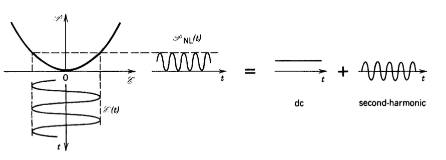
The figure illustrates how the square of the electric field leads to both the second harmonic generation (oscillating at 2ω) and optical rectification (the DC component) as previously derived mathematically. This visualization helps conceptualize how a single-frequency input creates multiple frequency components in the polarization response of a nonlinear medium.
Optical Rectification
Optical rectification is a second-order nonlinear process where an intense optical field generates a static (DC) polarization in a nonlinear medium. As previously noted in our discussion of SHG, when a monochromatic field is applied:
\[\mathbf{E}(t) = \mathbf{E}_\omega e^{-i\omega t} + \mathbf{E}_\omega^* e^{i\omega t}\]
The second-order polarization includes a DC term:
\[\mathbf{P}^{(2)}_{DC} = \varepsilon_0 \chi^{(2)} \cdot 2|\mathbf{E}_\omega|^2\]
This DC polarization is proportional to the intensity of the incident light. The direction of the induced polarization \(\mathbf{P}\) depends on the crystal structure through the second-order susceptibility tensor \(\chi^{(2)}\), which relates the components of \(\mathbf{P}\) to the square of \(\mathbf{E}\). More explicitly, we can write:
\[P_i^{(2)} = \varepsilon_0 \sum_{j,k} \chi_{ijk}^{(2)} E_j E_k\]
where the indices \(i\), \(j\), and \(k\) represent the Cartesian components. This tensorial relationship means that the polarization direction is not necessarily parallel to the electric field, but is determined by the symmetry properties of the nonlinear medium. Physically, optical rectification can be viewed as a process that “rectifies” the oscillating electric field of light into a static electric field.
One important application of optical rectification is the generation of terahertz (THz) radiation. When ultrashort laser pulses (with broad frequency spectra) undergo optical rectification, the resulting time-varying polarization can radiate electromagnetic waves in the THz region. This provides a convenient method for generating broadband THz radiation for spectroscopy and imaging applications.
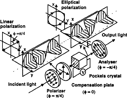
Electro-Optic Effect
The electro-optic effect, also known as the Pockels effect, can be derived from the second-order nonlinear mixing of an optical wave and a static electric field. Consider a total electric field consisting of an optical component at frequency \(\omega\) and a DC field:
\[\mathbf{E}(t) = \mathbf{E}_\omega e^{-i\omega t} + \mathbf{E}_\omega^* e^{i\omega t} + \mathbf{E}_{DC}\]
The second-order polarization in the nonlinear medium is:
\[\mathbf{P}^{(2)}(t) = \varepsilon_0 \chi^{(2)} \mathbf{E}^2(t)\]
Expanding this expression:
\[\mathbf{P}^{(2)}(t) = \varepsilon_0 \chi^{(2)} [\mathbf{E}_\omega^2 e^{-2i\omega t} + (\mathbf{E}_\omega^*)^2 e^{2i\omega t} + \mathbf{E}_{DC}^2 + 2|\mathbf{E}_\omega|^2 + 2\mathbf{E}_\omega \mathbf{E}_{DC} e^{-i\omega t} + 2\mathbf{E}_\omega^* \mathbf{E}_{DC} e^{i\omega t}]\]
The terms oscillating at frequency \(\omega\) are particularly significant as they modify the propagation of the optical wave:
\[\mathbf{P}^{(2)}_\omega = 2\varepsilon_0 \chi^{(2)} \mathbf{E}_\omega \mathbf{E}_{DC} e^{-i\omega t}\]
This adds to the linear polarization at frequency \(\omega\):
\[\mathbf{P}^{(1)}_\omega = \varepsilon_0 \chi^{(1)} \mathbf{E}_\omega e^{-i\omega t}\]
The total polarization at frequency \(\omega\) becomes:
\[\mathbf{P}_\omega = \varepsilon_0 [\chi^{(1)} + 2\chi^{(2)}\mathbf{E}_{DC}] \mathbf{E}_\omega e^{-i\omega t}\]
This can be viewed as a modification of the effective susceptibility due to the applied DC field:
\[\chi^{eff} = \chi^{(1)} + 2\chi^{(2)}\mathbf{E}_{DC}\]
Since the refractive index is related to susceptibility by \(n^2 = 1 + \chi\), we can directly calculate how the DC field changes the refractive index. For the case without a DC field, we have:
\[n_0^2 = 1 + \chi^{(1)}\]
When the DC field is applied, the effective refractive index becomes:
\[n^2 = 1 + \chi^{eff} = 1 + \chi^{(1)} + 2\chi^{(2)}\mathbf{E}_{DC}\]
This gives us:
\[n^2 = n_0^2 + 2\chi^{(2)}\mathbf{E}_{DC}\]
The change in refractive index is \(\Delta n = n - n_0\). We can express this as:
\[n = \sqrt{n_0^2 + 2\chi^{(2)}\mathbf{E}_{DC}}\]
For typical situations where the nonlinear effect is small compared to the linear refractive index (\(2\chi^{(2)}\mathbf{E}_{DC} \ll n_0^2\)), we can use the binomial approximation:
\[\sqrt{a + b} \approx \sqrt{a} + \frac{b}{2\sqrt{a}} \text{ when } b \ll a\]
Applying this approximation:
\[n \approx n_0 + \frac{2\chi^{(2)}\mathbf{E}_{DC}}{2n_0} = n_0 + \frac{\chi^{(2)}\mathbf{E}_{DC}}{n_0}\]
Therefore, the change in refractive index due to the DC field is:
\[\Delta n \approx \frac{\chi^{(2)}\mathbf{E}_{DC}}{n_0}\]
This direct relationship shows how the second-order nonlinear susceptibility couples with the DC electric field to modify the refractive index of the material.
The electro-optic effect enables several important devices:
- Electro-optic modulators: Used to modulate the amplitude, phase, or polarization of light
- Q-switches: For generating short, intense laser pulses
- Optical isolators: For preventing back-reflections in optical systems
- Pockels cells: For rapidly switching polarization states
Common electro-optic materials include lithium niobate (LiNbO₃), potassium dihydrogen phosphate (KDP), and various organic crystals.
Sum and Difference Frequency Generation
Sum and difference frequency generation is a natural extension of the electro-optic effect discussed earlier. While the electro-optic effect involved the interaction between a DC field and an optical wave, we now consider the interaction between two optical waves of different frequencies, allowing for the generation of new frequencies that are either the sum or difference of the input frequencies.
When two laser beams with frequencies \(\omega_1\) and \(\omega_2\) interact in a nonlinear medium, the total electric field can be written as:
\[\mathbf{E}(t) = \mathbf{E}_1 e^{-i\omega_1 t} + \mathbf{E}_2 e^{-i\omega_2 t} + c.c.\]
The second-order polarization is proportional to the square of this field. Expanding this expression:
\[\begin{align} \mathbf{P}^{(2)}(t) &= \varepsilon_0 \chi^{(2)} [ \\ &\mathbf{E}_1^2 e^{-2i\omega_1 t} + \mathbf{E}_2^2 e^{-2i\omega_2 t} + \\ &2\mathbf{E}_1\mathbf{E}_2 e^{-i(\omega_1+\omega_2) t} + 2\mathbf{E}_1\mathbf{E}_2^* e^{-i(\omega_1-\omega_2) t} + \\ &c.c. + 2|\mathbf{E}_1|^2 + 2|\mathbf{E}_2|^2] \end{align}\]
This expression contains several important terms:
- Second harmonic terms at \(2\omega_1\) and \(2\omega_2\)
- Sum frequency term at \(\omega_1 + \omega_2\) (from \(\mathbf{E}_1 \mathbf{E}_2 e^{-i(\omega_1+\omega_2)t}\))
- Difference frequency term at \(\omega_1 - \omega_2\) (from \(\mathbf{E}_1 \mathbf{E}_2^* e^{-i(\omega_1-\omega_2)t}\))
- DC terms from \(2|\mathbf{E}_1|^2\) and \(2|\mathbf{E}_2|^2\) (optical rectification)
While the electro-optic effect can be viewed as a special case where one of the fields is at zero frequency (DC), the sum and difference frequency generation involves two oscillating fields, creating new optical frequencies through their nonlinear interaction. This fundamental process enables frequency conversion across the electromagnetic spectrum and forms the basis for many applications, including infrared spectroscopy, tunable laser sources, and optical parametric amplifiers.
Optical Parametric Amplification and Oscillation
One of the most powerful and versatile applications of nonlinear optics is optical parametric amplification and oscillation. These processes enable the generation of tunable coherent light across spectral regions that are difficult or impossible to access with conventional lasers—a capability that has revolutionized fields from spectroscopy to quantum optics.
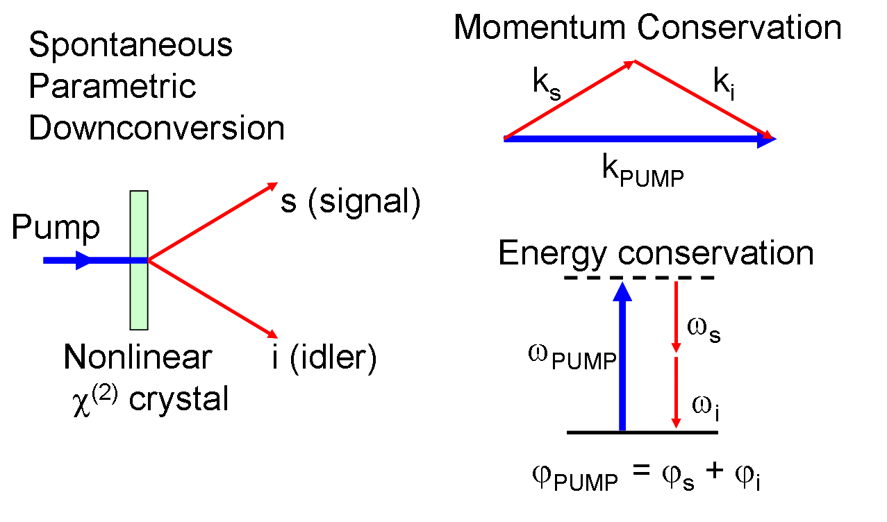
In optical parametric processes, a pump photon of frequency \(\omega_p\) splits into signal (\(\omega_s\)) and idler (\(\omega_i\)) photons, where \(\omega_p = \omega_s + \omega_i\). This can be viewed as the reverse of sum-frequency generation. What makes this process particularly valuable is that by adjusting phase-matching conditions through temperature tuning or crystal orientation, researchers can continuously select which frequencies are generated, effectively creating a “laser” whose output wavelength is tunable over an extremely broad range.
In the complex notation, this process is described by a polarization term:
\[\mathbf{P}^{(2)}(\omega_s) \propto \varepsilon_0 \chi^{(2)} \mathbf{E}_p \mathbf{E}_i^*\]
This term acts as a driving force that amplifies the signal field. When placed in a resonant cavity, this becomes an optical parametric oscillator (OPO), producing tunable output frequencies. Today, OPOs are indispensable tools in applications requiring mid-infrared light, including molecular spectroscopy, remote sensing, medical diagnostics, and as sources for nondestructive material testing where conventional laser sources are unavailable.
Spontaneous parametric downconversion (SPDC) represents the quantum mechanical limit of the parametric amplification process, where vacuum fluctuations stimulate the creation of photon pairs. In this process, a pump photon spontaneously converts into two lower-energy photons (signal and idler) within a nonlinear crystal, with no initial seed field required. This process is governed by the same energy conservation (\(\omega_p = \omega_s + \omega_i\)) and phase-matching (\(\mathbf{k}_p = \mathbf{k}_s + \mathbf{k}_i\)) conditions as classical parametric amplification.
What makes SPDC particularly significant for quantum information science is that the generated photon pairs exhibit quantum entanglement—a non-classical correlation that Einstein famously referred to as “spooky action at a distance.” The photons can be entangled in various degrees of freedom:
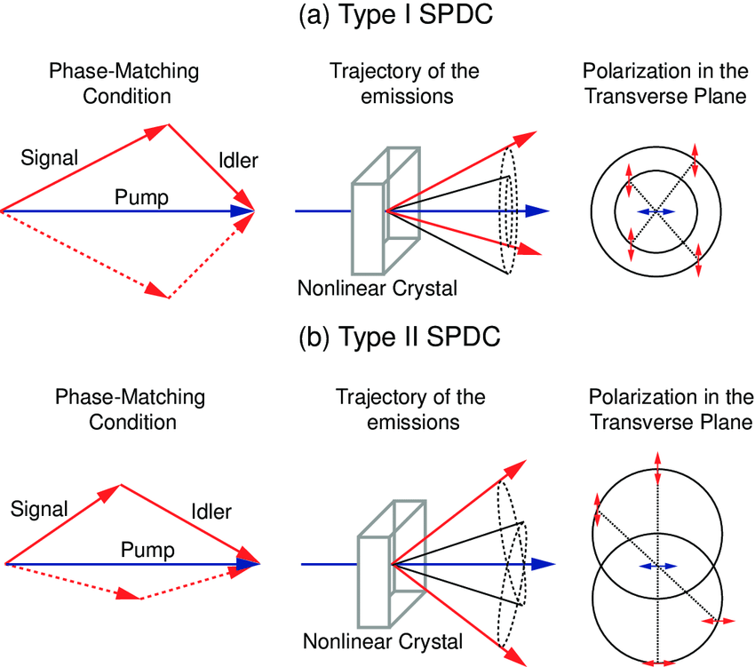
Polarization entanglement: The polarization states of the two photons are correlated such that measuring the polarization of one photon instantly determines the polarization of its partner, regardless of their separation distance. This can be achieved using Type-II phase matching where the signal and idler photons have orthogonal polarizations, and their emission cones overlap.
Momentum entanglement: The emission direction (wavevector) of one photon is correlated with that of its partner, constrained by the phase-matching conditions.
Energy-time entanglement: The exact time of photon pair creation is uncertain within the coherence time of the pump laser, leading to entanglement in the energy-time domain.
The quantum state of the generated photon pair can be written as:
\[|\Psi\rangle = \frac{1}{\sqrt{2}}(|H\rangle_s|V\rangle_i + e^{i\phi}|V\rangle_s|H\rangle_i)\]
for polarization-entangled photons, where \(|H\rangle\) and \(|V\rangle\) represent horizontal and vertical polarization states, and \(\phi\) is a relative phase that can be controlled experimentally.
Entangled photon sources based on SPDC have become foundational tools for quantum information processing, including:
- Quantum key distribution for secure communication
- Bell inequality tests for verification of quantum mechanics
- Quantum teleportation protocols
- Optical quantum computing experiments
- Quantum metrology and imaging with enhanced sensitivity
A typical experimental setup for generating polarization-entangled photons consists of a UV pump laser (often 405nm) illuminating a nonlinear crystal such as beta-barium borate (BBO). The downconverted photons pass through polarization optics and narrow-band filters before being collected into single-mode fibers connected to single-photon detectors. Coincidence counting electronics then identify the correlated photon pairs, confirming their entangled nature through quantum state tomography or Bell inequality measurements.
The efficiency of SPDC is typically quite low (approximately 10^-10 to 10^-8 pair generation probability per pump photon), but recent advances in periodically poled materials, waveguide structures, and cavity enhancement have significantly improved brightness and collection efficiency, making these sources increasingly practical for quantum technologies.
Three-Wave Mixing: A General Framework
All the second-order nonlinear processes we’ve discussed—second harmonic generation, optical rectification, electro-optic effect, sum and difference frequency generation, and optical parametric amplification—can be understood within a unified theoretical framework called three-wave mixing. This general approach provides deeper insight into the fundamental physics underlying these phenomena and reveals the common principles that govern their behavior.
The General Three-Wave Mixing Process
In three-wave mixing, three electromagnetic waves interact through the second-order nonlinear susceptibility \(\chi^{(2)}\) of a medium. These three waves, with frequencies \(\omega_1\), \(\omega_2\), and \(\omega_3\), are coupled through the nonlinear polarization. The key insight is that energy and momentum conservation require:
Energy Conservation (Photon Picture): \[\omega_3 = \omega_1 + \omega_2\]
Momentum Conservation (Phase Matching): \[\mathbf{k}_3 = \mathbf{k}_1 + \mathbf{k}_2\]
where \(\mathbf{k}_i = n_i \omega_i / c\) are the wave vectors of the three waves.
Coupled Wave Equations
The evolution of the three interacting waves can be described by a set of coupled differential equations. Starting from Maxwell’s equations with the nonlinear polarization as a source term, we can derive:
\[\frac{dA_1}{dz} = -i\frac{\omega_1 d_\text{eff}}{n_1 c} A_2^* A_3 e^{i\Delta k z}\]
\[\frac{dA_2}{dz} = -i\frac{\omega_2 d_\text{eff}}{n_2 c} A_1^* A_3 e^{i\Delta k z}\]
\[\frac{dA_3}{dz} = -i\frac{\omega_3 d_\text{eff}}{n_3 c} A_1 A_2 e^{-i\Delta k z}\]
where \(A_i\) are the slowly varying amplitudes of the three waves, \(d_\text{eff}\) is the effective nonlinear coefficient, and \(\Delta k = k_3 - k_1 - k_2\) is the phase mismatch.
To derive these coupled wave equations:
Start with Maxwell’s wave equation including the nonlinear polarization: \[\nabla^2 \mathbf{E} - \frac{n^2}{c^2} \frac{\partial^2 \mathbf{E}}{\partial t^2} = \mu_0 \frac{\partial^2 \mathbf{P}^{NL}}{\partial t^2}\]
Express the total electric field as a sum of three waves: \[\mathbf{E}(z,t) = \frac{1}{2}\sum_{j=1}^{3} [A_j(z) e^{i(k_j z - \omega_j t)} + c.c.]\] where \(A_j(z)\) are slowly varying amplitudes.
The second-order nonlinear polarization is: \[\mathbf{P}^{(2)}(z,t) = \varepsilon_0 \chi^{(2)} \mathbf{E}^2(z,t)\]
For each frequency component \(\omega_j\), extract the relevant polarization term:
- For \(\omega_1\): \(\mathbf{P}^{(2)}(\omega_1) \propto \varepsilon_0 \chi^{(2)} A_2^* A_3 e^{i[(k_3-k_2)z - \omega_1 t]}\)
- For \(\omega_2\): \(\mathbf{P}^{(2)}(\omega_2) \propto \varepsilon_0 \chi^{(2)} A_1^* A_3 e^{i[(k_3-k_1)z - \omega_2 t]}\)
- For \(\omega_3\): \(\mathbf{P}^{(2)}(\omega_3) \propto \varepsilon_0 \chi^{(2)} A_1 A_2 e^{i[(k_1+k_2)z - \omega_3 t]}\)
Substitute into the wave equation and apply the slowly varying amplitude approximation: \[\left|\frac{d^2 A_j}{dz^2}\right| \ll \left|k_j \frac{dA_j}{dz}\right|\]
Define \(\Delta k = k_3 - k_1 - k_2\) and the effective nonlinear coefficient \(d_{eff} = \frac{1}{2}\chi^{(2)}\)
After simplification, we obtain the three coupled equations: \[\frac{dA_1}{dz} = -i\frac{\omega_1 d_\text{eff}}{n_1 c} A_2^* A_3 e^{i\Delta k z}\]
\[\frac{dA_2}{dz} = -i\frac{\omega_2 d_\text{eff}}{n_2 c} A_1^* A_3 e^{i\Delta k z}\]
\[\frac{dA_3}{dz} = -i\frac{\omega_3 d_\text{eff}}{n_3 c} A_1 A_2 e^{-i\Delta k z}\]
These equations describe the energy exchange between the three waves and form the foundation for analyzing all three-wave mixing processes.
Unifying Second-Order Processes
This general framework elegantly encompasses all the second-order processes we’ve studied:
- Second Harmonic Generation: Set \(\omega_1 = \omega_2 = \omega\) and \(\omega_3 = 2\omega\)
- Optical Rectification: Set \(\omega_1 = \omega\), \(\omega_2 = -\omega\), and \(\omega_3 = 0\) (DC)
- Electro-Optic Effect: Set \(\omega_1 = 0\) (DC field), \(\omega_2 = \omega\), and \(\omega_3 = \omega\)
- Sum Frequency Generation: All three frequencies are different with \(\omega_3 = \omega_1 + \omega_2\)
- Difference Frequency Generation: Set \(\omega_2 = -\omega_2'\) so that \(\omega_3 = \omega_1 - \omega_2'\)
- Optical Parametric Amplification: Pump at \(\omega_3\) generates signal at \(\omega_1\) and idler at \(\omega_2\)
Energy Flow and Conservation
The coupled wave equations reveal that energy flows between the three waves in a way that conserves total energy. The Manley-Rowe relations, derived from these equations, show that:
\[\frac{1}{\omega_1}\frac{d}{dz}\left(\frac{|A_1|^2}{2}\right) + \frac{1}{\omega_3}\frac{d}{dz}\left(\frac{|A_3|^2}{2}\right) = 0\]
\[\frac{1}{\omega_2}\frac{d}{dz}\left(\frac{|A_2|^2}{2}\right) + \frac{1}{\omega_3}\frac{d}{dz}\left(\frac{|A_3|^2}{2}\right) = 0\]
These relations ensure that the number of photons is conserved in the interaction: when one photon at \(\omega_3\) is destroyed, one photon each at \(\omega_1\) and \(\omega_2\) is created, and vice versa.
The Role of Phase Matching
The exponential factor \(e^{i\Delta k z}\) in the coupled wave equations reveals a critical requirement for efficient nonlinear interactions: phase matching, where \(\Delta k \approx 0\). Phase matching ensures that the nonlinear polarization and the generated electromagnetic wave maintain proper phase alignment throughout the propagation distance. When perfectly phase-matched (\(\Delta k = 0\)), the energy transfer between interacting waves accumulates constructively along the entire crystal length, maximizing conversion efficiency. Without phase matching (\(\Delta k \neq 0\)), the direction of energy flow oscillates with a coherence length \(L_c = \pi/|\Delta k|\), severely limiting the effective interaction length and conversion efficiency.
Several techniques have been developed to achieve phase matching:
Birefringent phase matching: This technique exploits the refractive index difference between orthogonal polarization states in anisotropic crystals. By carefully orienting the crystal and selecting appropriate polarizations, one can satisfy the condition \(n_1(\omega_1) = n_3(\omega_3)\) for type-I phase matching or other analogous conditions for different processes. Temperature tuning can provide fine adjustment of these conditions in many materials.
Quasi-phase matching: When birefringent phase matching is difficult or impossible, quasi-phase matching offers an elegant alternative. Rather than maintaining \(\Delta k = 0\), this approach periodically inverts the sign of the nonlinear coefficient (typically by creating periodic domain inversions in ferroelectric materials) with period \(\Lambda = 2L_c\). This effectively resets the phase relationship at precisely the distance where destructive interference would begin, allowing efficient nonlinear conversion even in materials that cannot be birefringently phase-matched.
Modal phase matching: In waveguides and fibers, the different propagation constants of various spatial modes can be exploited to achieve phase matching between waves of different frequencies traveling in different modes.
Third-Order Nonlinear Processes
Third-order nonlinear processes arise from the third-order susceptibility \(\chi^{(3)}\) and represent a fundamentally different class of optical phenomena compared to second-order effects. While second-order processes require non-centrosymmetric materials and involve three-wave mixing, third-order effects can occur in all materials, including centrosymmetric crystals, glasses, and liquids, making them universally accessible across a broad range of optical materials.
Experimental Identification through Intensity Dependence
Third-order nonlinear processes are characterized by their cubic dependence on the incident laser intensity. The third-order polarization is given by:
\[\mathbf{P}^{(3)} = \varepsilon_0 \chi^{(3)} \mathbf{E}^3\]
Since intensity \(I \propto |\mathbf{E}|^2\), the nonlinear signal scales as:
\[I_{signal} \propto I^3\]
This scaling is verifiable by measuring the slope on a log-log plot of signal versus input power. The strong intensity dependence makes third-order effects prominent in ultrafast optics and high-intensity laser applications, enabling phenomena such as four-wave mixing, intensity-dependent refractive indices, and self-action effects.
Third Harmonic Generation
Third harmonic generation (THG) is the simplest third-order frequency conversion process, where three photons at frequency \(\omega\) combine to produce one photon at frequency \(3\omega\). Unlike second harmonic generation, THG can occur in any material since it doesn’t require the breaking of inversion symmetry.
For a monochromatic wave \(\mathbf{E}(t) = \mathbf{E}_0 e^{-i\omega t} + c.c.\), the third-order polarization contains a term:
\[\mathbf{P}^{(3)}(3\omega) = \varepsilon_0 \chi^{(3)} \mathbf{E}_0^3 e^{-3i\omega t}\]
This polarization oscillates at \(3\omega\) and can drive the generation of third harmonic radiation. The conversion efficiency depends on the cube of the incident intensity, making THG particularly sensitive to peak power. This cubic dependence means that THG is most efficient with ultrashort, high-intensity pulses.
The phase matching condition for THG is:
\[\Delta k = k_{3\omega} - 3k_{\omega} = 0\]
where \(k_{\omega} = n(\omega)\omega/c\) and \(k_{3\omega} = n(3\omega)3\omega/c\). Due to normal dispersion, this condition is typically not satisfied in bulk materials, but can be achieved in specially designed waveguides or by using focused beams where the Gouy phase shift can compensate for the material dispersion.
THG is widely used in microscopy applications, particularly for biological imaging, because it provides excellent depth resolution and can penetrate deeper into tissues than two-photon fluorescence. The technique is also valuable for characterizing ultrashort pulses and for generating UV light from near-infrared sources.
Intensity-Dependent Refractive Index (Kerr Effect)
One of the most important third-order nonlinear effects is the intensity-dependent refractive index, also known as the optical Kerr effect. This phenomenon occurs because the third-order polarization includes a term that oscillates at the same frequency as the driving field, effectively modifying the material’s linear response.
For a field \(\mathbf{E}(t) = \mathbf{E}_0 e^{-i\omega t} + c.c.\), the third-order polarization includes:
\[\mathbf{P}^{(3)}(\omega) = 3\varepsilon_0 \chi^{(3)} |\mathbf{E}_0|^2 \mathbf{E}_0 e^{-i\omega t}\]
This term is proportional to the intensity \(I = (n\varepsilon_0 c/2)|\mathbf{E}_0|^2\) and modifies the effective susceptibility. The resulting refractive index becomes:
\[n = n_0 + n_2 I\]
where \(n_0\) is the linear refractive index and \(n_2\) is the nonlinear refractive index coefficient:
\[n_2 = \frac{3\operatorname{Re}(\chi^{(3)})}{2n_0^2\varepsilon_0 c}\]
The sign of \(n_2\) depends on the material: most common optical materials have \(n_2 > 0\) (self-focusing), while some materials exhibit \(n_2 < 0\) (self-defocusing). The magnitude of \(n_2\) varies dramatically between materials, from \(10^{-20}\) m²/W in silica glass to \(10^{-17}\) m²/W in some semiconductors.
This intensity-dependent refractive index is the foundation for many important nonlinear optical phenomena, including self-phase modulation, self-focusing, and soliton formation in optical fibers.
Four-Wave Mixing
Four-wave mixing (FWM) is a third-order nonlinear process where four photons interact through the material’s \(\chi^{(3)}\) susceptibility. The general energy conservation condition is:
\[\omega_1 + \omega_2 = \omega_3 + \omega_4\]
with corresponding momentum conservation:
\[\mathbf{k}_1 + \mathbf{k}_2 = \mathbf{k}_3 + \mathbf{k}_4\]
Consider two strong pump waves at frequencies \(\omega_1\) and \(\omega_2\), and weaker signal and idler waves at \(\omega_3\) and \(\omega_4\). The coupled wave equations for the signal and idler amplitudes are:
\[\frac{dA_3}{dz} = i\gamma A_1 A_2 A_4^* e^{i\Delta k z}\]
\[\frac{dA_4}{dz} = i\gamma A_1 A_2 A_3^* e^{i\Delta k z}\]
where \(\gamma = \omega n_2/(cA_{eff})\) is the nonlinear coefficient and \(A_{eff}\) is the effective mode area.
Special cases of four-wave mixing include:
Degenerate Four-Wave Mixing: When \(\omega_1 = \omega_2 = \omega_p\) (pump frequency), the process becomes \(2\omega_p = \omega_s + \omega_i\), where a strong pump generates signal and idler waves symmetrically placed around the pump frequency.
Stimulated Raman Scattering: A special case where energy conservation is satisfied through molecular vibrations, leading to frequency downshift by the Raman shift.
Phase Conjugation: When \(\omega_1 = \omega_3\) and \(\omega_2 = \omega_4\), the process can generate a phase-conjugated replica of an input beam.
Four-wave mixing is extensively used in fiber optics for wavelength conversion, optical parametric amplification, and supercontinuum generation. It’s also the basis for many all-optical signal processing applications.
Self-Phase Modulation and Self-Focusing
Self-phase modulation (SPM) and self-focusing are two closely related phenomena that arise from the intensity-dependent refractive index. Both effects demonstrate how intense light can modify its own propagation characteristics.
Self-Phase Modulation
In self-phase modulation, the intensity-dependent refractive index causes the phase of a propagating wave to depend on its own intensity. For a pulse with temporally varying intensity \(I(t)\), the accumulated phase after propagation distance \(z\) is:
\[\phi(t) = \frac{\omega z}{c}[n_0 + n_2 I(t)] = \phi_0 + \phi_{NL}(t)\]
The nonlinear phase \(\phi_{NL}(t) = \omega z n_2 I(t)/c\) varies with time, leading to an instantaneous frequency shift:
\[\omega_{inst}(t) = \omega_0 - \frac{d\phi_{NL}}{dt} = \omega_0 - \frac{\omega z n_2}{c}\frac{dI}{dt}\]
This creates new frequency components: the leading edge of the pulse (where \(dI/dt > 0\)) is red-shifted, while the trailing edge (where \(dI/dt < 0\)) is blue-shifted. For \(n_2 > 0\), this leads to significant spectral broadening while preserving the pulse energy.
SPM is crucial for supercontinuum generation, where the combination of SPM and dispersion in optical fibers creates extremely broad spectral bandwidth from narrow-band input pulses.
Self-Focusing
Self-focusing occurs when the intensity-dependent refractive index creates a transverse gradient that acts like a positive lens. For a Gaussian beam with peak intensity \(I_0\), the on-axis refractive index is higher than at the beam edges, creating a waveguide effect.
The critical power for self-focusing is:
\[P_{crit} = \frac{\lambda^2}{2\pi n_0 n_2}\]
When the beam power exceeds \(P_{crit}\), the nonlinear focusing effect overcomes natural diffraction, leading to catastrophic beam collapse. In practice, this process is limited by other nonlinear effects like multiphoton absorption or material breakdown.
Self-focusing is both useful and problematic: it can enhance nonlinear interactions by increasing intensity, but it can also damage optical materials and limit the power handling capability of optical systems.
These third-order effects are fundamental to many applications in modern photonics, including ultrafast optics, optical communications, and materials processing. Their universal occurrence in all materials makes them particularly important for developing nonlinear optical devices and understanding high-intensity light propagation.
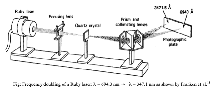
Frequency conversion (lasers of new colors): Nonlinear frequency conversion enables the generation of laser light at wavelengths that are difficult or impossible to achieve with conventional laser gain media. For example, green laser pointers typically use a 1064nm infrared laser with frequency doubling in a nonlinear crystal to produce 532nm green light. This capability has revolutionized laser technology by vastly expanding the available wavelength range.
Optical parametric oscillators for tunable light sources: OPOs provide continuously tunable coherent radiation across spectral regions from the visible to the mid-infrared. This tunability is crucial for spectroscopy, sensing applications, and quantum optics where specific wavelengths are required to interact with particular molecular transitions or quantum systems.
Ultrashort pulse generation: Nonlinear effects like Kerr lens mode-locking and saturable absorption enable the generation of femtosecond and even attosecond pulses. These ultrashort pulses allow scientists to observe and manipulate ultrafast phenomena like chemical reactions, electron dynamics, and molecular vibrations in real-time.
Optical switching and computing: The intensity-dependent properties of nonlinear materials enable all-optical switching without conversion to electronic signals. This capability is foundational for future photonic computing architectures that promise much higher speeds and lower power consumption than electronic equivalents.
Optical limiting for protection against intense light: Materials with nonlinear absorption can protect sensitive optical sensors and human eyes from damage by intense laser light. These materials become increasingly opaque as the incident intensity increases, providing automatic protection against optical damage.
Imaging techniques like second-harmonic generation microscopy: SHG microscopy provides label-free imaging of non-centrosymmetric structures like collagen fibers in biological tissues. This technique offers high contrast, three-dimensional resolution, and minimal photodamage compared to conventional fluorescence microscopy, making it invaluable for biomedical research.
Typical Materials for Nonlinear Optics
Lithium Niobate (LiNbO₃): A versatile ferroelectric crystal with large electro-optic and nonlinear coefficients. It’s widely used for frequency doubling, parametric oscillation, and electro-optic modulation. Periodically poled lithium niobate (PPLN) enables efficient quasi-phase-matched interactions across a broad wavelength range.
Potassium Dihydrogen Phosphate (KDP): An inexpensive crystal with good UV transparency, commonly used for frequency doubling and Pockels cells. It can be grown in large sizes with high optical quality, making it suitable for high-power laser systems.
Beta Barium Borate (BBO): Features a wide transparency range (189-3500nm) and high damage threshold, making it excellent for UV generation and ultrafast applications. Its large birefringence allows phase matching across a broad spectral range.
Gallium Arsenide (GaAs): A semiconductor with extremely high nonlinear coefficients, useful for mid-infrared applications. GaAs waveguides and orientation-patterned structures enable efficient nonlinear interactions at relatively low powers.
Silica fibers (for third-order effects): While silica has modest nonlinear coefficients, the long interaction lengths and tight confinement in optical fibers enhance nonlinear effects like self-phase modulation, four-wave mixing, and stimulated Raman scattering.
Typical Experimental Setup
Laser source (typically pulsed for high intensity): High peak intensities are essential for efficient nonlinear interactions. Mode-locked Ti:Sapphire lasers, fiber lasers, and Q-switched Nd:YAG systems are common choices depending on the application requirements.
Focusing optics: Properly designed lens systems concentrate the laser energy to achieve the necessary intensity while optimizing the beam size throughout the nonlinear medium for phase matching and avoiding damage.
The nonlinear medium: Often mounted on a precision rotation stage for angle tuning, and sometimes in a temperature-controlled oven for temperature tuning of phase matching conditions. Crystal orientation, temperature, and sometimes applied electric fields are adjusted to optimize the desired nonlinear process.
Filters to select the desired output frequency: Dichroic mirrors, prisms, or gratings separate the generated nonlinear signal from the fundamental beam and any other unwanted frequencies generated in the nonlinear process.
Detection and measurement equipment ::: modulation techniques. often employed for weak signal detection using-in amplifiers arelinear output. Lock temporal, and spatial properties of the nonize the spectral,odes, and cameras character, power meters, photodi: Spectrometers