When light enters a piece of glass, remarkable things happen: it bends, partially reflects, and travels at a different speed. These everyday phenomena - from the sparkle of a diamond to the operation of optical fibers - all stem from the fundamental interaction between electromagnetic waves and matter at the atomic level.
In this lecture, we’ll trace the complete story from individual atoms responding to electric fields to the macroscopic optical properties we observe and exploit in modern technology. We’ll see how:
Microscopic: Individual atoms become polarized in electric fields
Mesoscopic: Collections of atoms create bulk material properties
Macroscopic: Materials exhibit refractive indices and reflection/refraction
Applications: These principles enable countless optical technologies
Microscopic Origins - How Atoms Respond to Light
The Atomic Picture
To understand why materials affect light propagation, we start with individual atoms. Our simple but powerful model consists of:
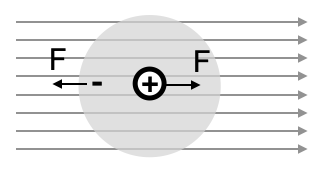
A positive nucleus at the center
A negative electron cloud of charge \(-q\) distributed in a sphere of radius \(a\)
An applied electric field that can displace these charges
Figure 1— Atomic polarization: An external electric field displaces the positive nucleus relative to the negative electron cloud, creating an induced dipole moment.
But what is \(\vec{E}_{\text{local}}\)? In dense materials, each atom feels not just the applied field but also fields from neighboring dipoles.
Maxwell’s Equations in Matter
From the polarization density \(\vec{P} = N\vec{p}\) we established earlier, we can now understand how this microscopic response modifies the macroscopic electromagnetic fields. The polarization creates bound charges within the material that must be accounted for in Maxwell’s equations.
The key insight is that the polarization \(\vec{P}\) represents dipole moments per unit volume, which creates a bound charge density:
\[\rho_b = -\nabla \cdot \vec{P}\]
To handle both free charges (from external sources) and bound charges (from polarization) in a unified way, we introduce the displacement field:
\[\vec{D} = \epsilon_0\vec{E} + \vec{P}\]
This displacement field allows us to write Gauss’s law in terms of only the free charge density \(\rho_f\), effectively “absorbing” the bound charges into the definition of \(\vec{D}\).
For linear materials, the polarization is proportional to the electric field:
\[\vec{P} = \epsilon_0\chi\vec{E}\]
where \(\chi\) is the electric susceptibility of the material. This gives us:
\[\nabla\cdot \vec{B}=0 \quad \text{(No magnetic monopoles)}\]
For linear materials: \(\vec{D}=\epsilon(\omega)\vec{E}\) and \(\vec{B}=\mu(\omega)\vec{H}\), where the frequency dependence is now explicit.
Local Field Effects: The Clausius-Mossotti Relation
When we try to connect the microscopic polarizability of individual atoms to macroscopic dielectric properties, we face a crucial problem: in dense materials, atoms don’t just experience the externally applied electric field. Instead, each atom sits in a complex field environment created by all other polarized atoms in the material.
To solve this problem, Lorentz developed a spherical cavity model. Consider a single atom at the center of a small spherical cavity within a uniformly polarized material. The local electric field experienced by this atom has three contributions:
\(\vec{E}\) is the macroscopic electric field (averaged over many atoms)
\(\vec{E}_{\text{depolarization}}\) is the field from polarization charges on the cavity surface
\(\vec{E}_{\text{near-field}}\) is from nearby dipoles within the cavity
For an idealized spherical cavity in a uniformly polarized medium, the near-field contribution vanishes due to symmetry. The depolarization field can be calculated from electrostatics:
This is the Clausius-Mossotti relation, a remarkable bridge between the microscopic world of atomic polarizability and the macroscopic world of dielectric constants. It successfully explains the refractive indices of many gases and liquids, though it becomes less accurate for strongly polar materials where dipole-dipole interactions become significant.
Wave Propagation and the Refractive Index
Wave Propagation and the Refractive Index
Combining Maxwell’s equations for source-free regions gives the wave equation in matter:
For non-magnetic materials (\(\mu_r=1\)), the refractive index is:
\[n=\frac{c}{v}=\sqrt{\epsilon_r}\]
When electromagnetic waves travel through a material, they interact with the bound charges (electrons and nuclei) we discussed earlier in the atomic polarization model. These microscopic interactions manifest as macroscopic modifications to the wave’s properties through a collective response of billions of atomic dipoles. Let’s examine these effects from a fundamental physical perspective.
Phase Velocity and Wavelength Changes
In a material with refractive index \(n\), the phase velocity of light becomes:
\[v_p = \frac{c}{n}\]
This reduction in velocity isn’t just a mathematical relationship - it has a direct physical cause. As the electromagnetic wave propagates, it induces oscillating dipoles in the material’s atoms. These oscillating dipoles temporarily store electromagnetic energy and re-emit it with a phase delay. This cyclic process of absorption and re-emission effectively increases the time it takes for the wave to propagate through the medium, reducing its effective velocity.
The wavelength must change inside the material while the frequency remains constant (since frequency is determined by the source and must match at boundaries):
This wavelength reduction can be understood as spatial compression of the wavefronts: since the wave oscillates at the same frequency but travels more slowly, the distance between successive crests must decrease proportionally.
Mathematical Description from First Principles
For a plane wave entering a material with refractive index \(n\), we can derive the behavior by considering how the material’s polarization response modifies the wave equation.
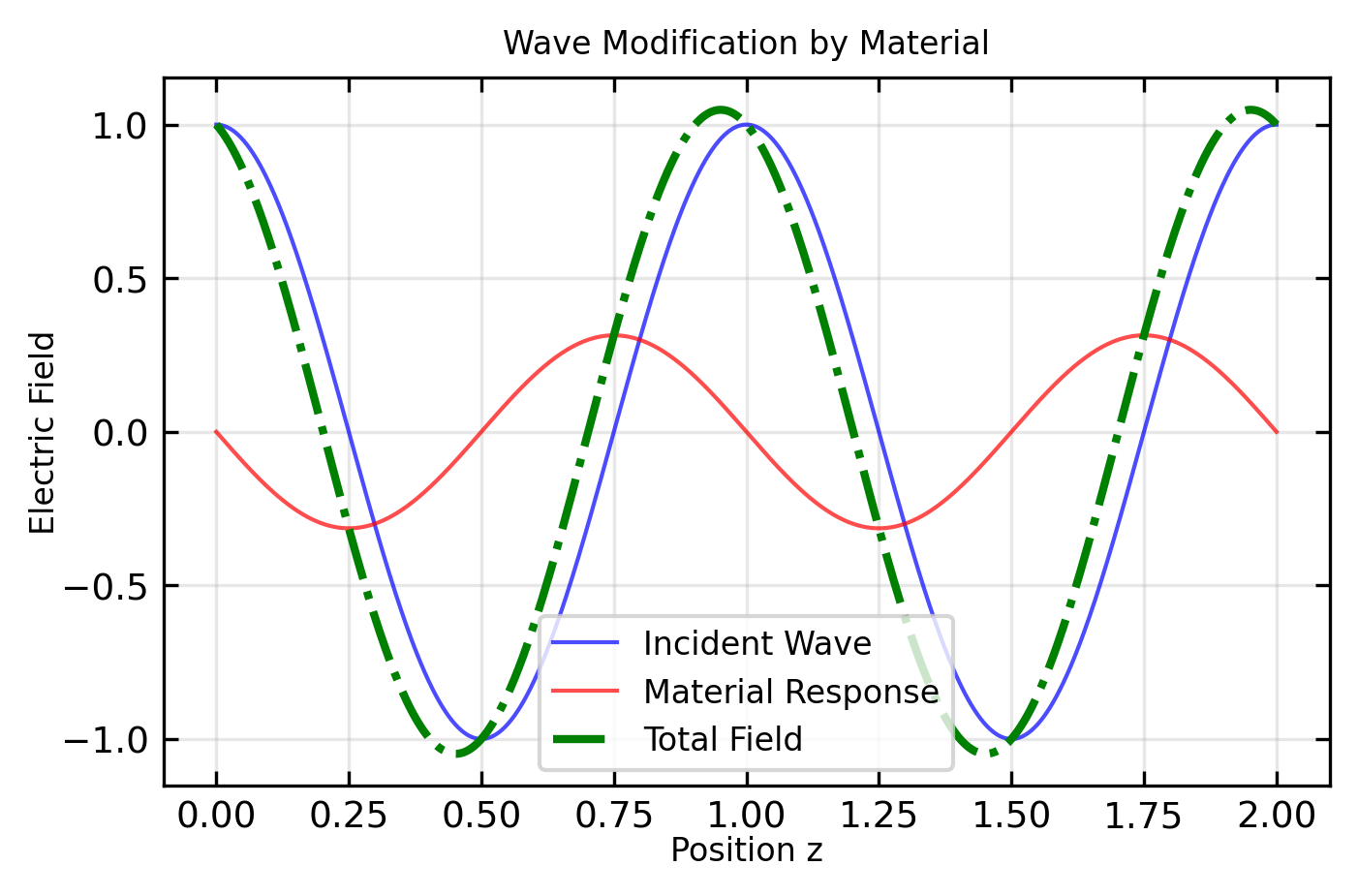
When passing through a thin material slab of thickness \(\Delta z\), the total field is a superposition of the incident wave and the field generated by the material’s polarization:
\[\begin{aligned}
E &= E_0 e^{i(\omega t - k z)} + E_{pol} \\
&= E_0 e^{i(\omega t - k z)} + E_0 e^{i(\omega t - k z)}(e^{-i(n-1)k\Delta z} - 1) \\
&= E_0 e^{i(\omega t - k z - (n-1)k\Delta z)} \\
&= E_0 e^{-i(n-1)k\Delta z} e^{i(\omega t - kz)} \\
&= E_0 e^{-i\phi} e^{i(\omega t - kz)}
\end{aligned}\]
where \(\phi = (n-1)k\Delta z\) is the phase shift introduced by the material. This phase shift has a direct physical interpretation: \((n-1)\) represents the additional optical path length per unit physical length caused by the material’s polarization response, and \(k\Delta z\) is the phase accumulated over distance \(\Delta z\).
Figure 2— Wave propagation through a thin material slab
Physical Interpretation at the Atomic Level
The physical mechanism behind wave modification in materials can be traced directly to our earlier discussion of atomic polarization. When an electromagnetic wave enters a material:
The wave’s electric field displaces electrons relative to nuclei, creating oscillating atomic dipoles at the frequency of the incident wave
These oscillating dipoles act as secondary sources, radiating their own electromagnetic waves according to Maxwell’s equations
The secondary waves combine with the incident wave through superposition, resulting in:
A phase shift (effectively delaying the wave)
A modified wave amplitude
Cancellation of backward-propagating components in the absence of reflections
The phase delay fundamentally results from the time lag in the atomic response. When the electric field pushes on the bound electrons, they don’t respond instantaneously but slightly lag the driving field (like a driven harmonic oscillator). This microscopic delay, multiplied across billions of atoms, creates the macroscopic effect of reduced phase velocity.
For a thick material (much greater than a wavelength), these phase shifts accumulate. In a 1 mm thick glass plate (\(n = 1.5\)) illuminated with visible light (\(\lambda = 500\) nm), the total phase shift is \((1.5-1) \times 2\pi \times \frac{10^{-3}}{500 \times 10^{-9}} \approx 6,280\) radians or about 1,000 complete cycles!
Group Velocity and Resonance Effects
The atomic perspective becomes especially important when considering wave packets rather than infinite plane waves. The group velocity governs the propagation of these packets:
This formula has a direct physical interpretation: when a material’s refractive index varies with wavelength (dispersion), different frequency components of a wave packet travel at different phase velocities. This happens because different frequencies excite the atomic dipoles with varying efficiencies depending on how close they are to the natural resonant frequencies of the material’s electrons.
In materials with normal dispersion (\(\frac{dn}{d\lambda} < 0\)), which occurs away from resonances, higher frequencies (shorter wavelengths) experience higher refractive indices because they drive the electrons more efficiently. Near atomic or molecular resonances, anomalous dispersion occurs, leading to dramatic changes in wave propagation and absorption.
The dispersion relation directly connects to the Lorentz-Drude model discussed later, where the refractive index emerges from treating the electrons as damped harmonic oscillators responding to the oscillating electric field of light.
Experimental Manifestations and Applications
The material modification of wave propagation manifests in numerous experimental observations and technologies:
Interference phenomena: In a Michelson interferometer, a thin glass plate inserted in one arm shifts the fringe pattern precisely because of the accumulated phase shift \(\phi = (n-1)k\Delta z\). This allows for extremely sensitive measurements of refractive indices or material thicknesses.
Optical path length: The concept of optical path length \(L_{opt} = nL_{physical}\) accounts for the additional phase accumulation in materials and is essential for designing optical systems from microscopes to telescopes.
Pulse dispersion: In optical communications, the wavelength dependence of refractive index causes different frequency components of pulses to travel at different velocities. This dispersion effect limits data transmission rates in fiber optic systems and requires compensation techniques.
Phase contrast microscopy: This Nobel Prize-winning technique exploits the phase shifts introduced by biological samples to convert otherwise invisible phase variations into visible intensity changes, revolutionizing biological imaging without needing stains.
The fundamental interaction between electromagnetic waves and bound charges thus bridges atomic physics to practical applications, demonstrating how microscopic quantum mechanical phenomena scale up to create macroscopic optical effects we can harness in technology.
Frequency Dependence of the Refractive Index: The Lorentz Oscillator Model
In the earlier atomic polarizability model, we treated atoms as static systems responding to a constant electric field. In reality, light consists of time-varying electromagnetic fields, and atoms respond dynamically to these oscillations. This frequency dependence fundamentally explains dispersion, absorption, and many optical phenomena.
From Static to Dynamic Atomic Response
Extending our previous atomic model, we now treat the electron as a damped harmonic oscillator driven by an oscillating electric field. For visible light (\(\lambda \approx 500\, \text{nm}\)) interacting with atoms (size \(\approx 0.1\, \text{nm}\)), we can make the dipole approximation where the field appears uniform across each atom (\(\vec{E}(\vec{r},t) \approx \vec{E}(t)\)), and the local field approximation where the field acting on each atom is approximately the macroscopic field (\(\vec{E}_\text{local} \approx \vec{E}\)).
For a harmonically oscillating electric field \(\vec{E}(t)=E_0\hat{x} e^{-i\omega t}\), the bound electron moves under the combined influence of the restoring force from the nucleus, damping from radiation and collisions, and the driving force from the electric field. This gives us the equation of motion: \[
m\ddot{\vec{r}}+m\sigma\dot{\vec{r}}+m\omega_0^2\vec{r}=q\vec{E}(t)
\]
Here, \(\omega_0\) is the natural resonance frequency of the electron, \(\sigma\) is the damping coefficient, \(q\) is the electron charge, and \(m\) is the electron mass.
Frequency-Dependent Polarizability
Solving this differential equation for a steady-state response, the electron displacement follows the driving field with frequency \(\omega\): \[
\vec{r}(t)=\frac{q/m}{\omega_0^2+i\omega\sigma-\omega^2}\vec{E}(t)
\]
From this, the frequency-dependent dipole moment becomes \(\vec{p}(\omega)=q\vec{r}(t)=\alpha(\omega)\vec{E}(t)\), where \(\alpha(\omega)=\frac{q^2/m}{\omega_0^2+i\omega\sigma-\omega^2}\) is the frequency-dependent polarizability. This directly extends our previous static model, with the atomic polarizability we derived earlier (\(\alpha=4\pi\epsilon_0 a^3\)) being approximately the low-frequency limit (\(\omega \rightarrow 0\)) of this more general expression.
From Polarizability to Complex Refractive Index
The macroscopic polarization density for \(N\) atoms per unit volume becomes
where \(\chi_0=\frac{Nq^2}{m\epsilon_0}\) represents the strength of the resonance.
Since the susceptibility is complex (\(\chi=\chi'+i\chi''\)), both the dielectric function \(\epsilon_r(\omega)=1+\chi(\omega)\) and the refractive index become complex quantities:
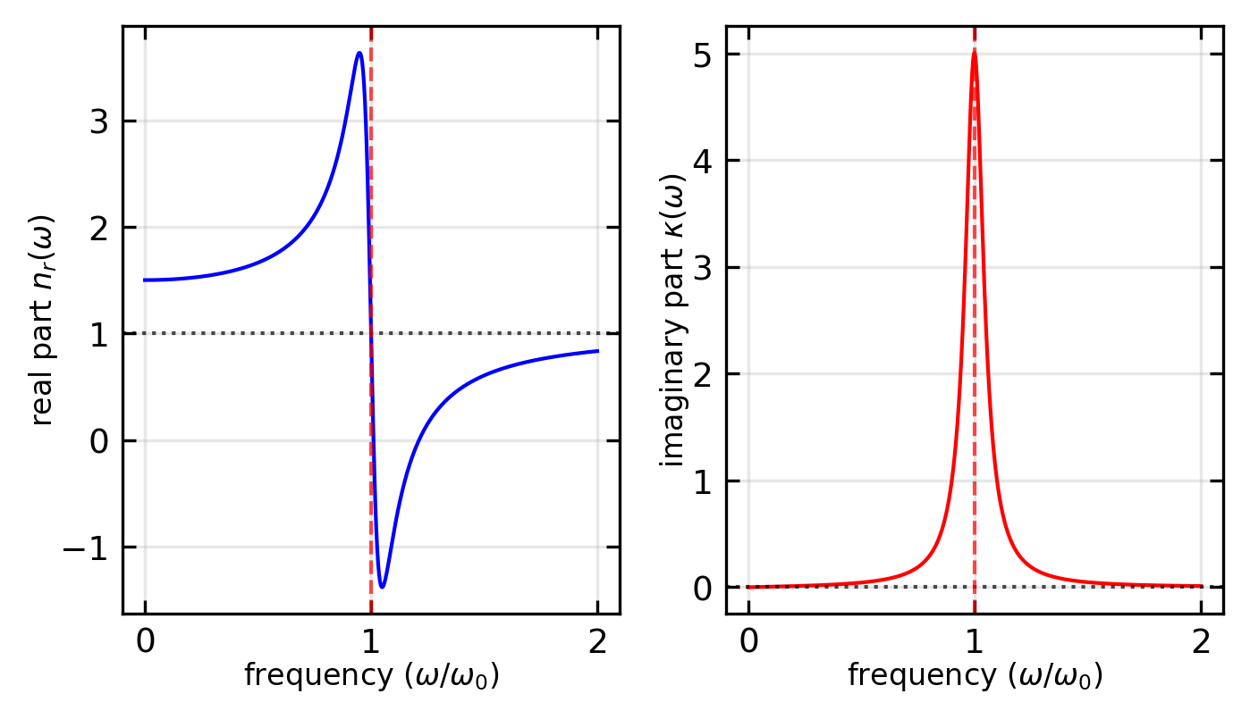
The real part \(n_r(\omega)\) controls the phase velocity and refraction, while the imaginary part \(\kappa(\omega)\) determines absorption according to the Beer-Lambert law: \(I \propto e^{-2\omega\kappa z/c}\). These components can be written as: \[n_r(\omega) = 1 + A\frac{(\omega_0^2-\omega^2)}{(\omega_0^2-\omega^2)^2+\omega^2\sigma^2}\]
Frequency dependence of refractive index near a resonance. The real part shows dispersion behavior around the resonance, while the imaginary part peaks at resonance, corresponding to maximum absorption.
Physical Interpretation and Applications
The plots above reveal how refractive index varies with frequency around a resonance. Below resonance (\(\omega < \omega_0\)), the real part exceeds 1 and increases with frequency (normal dispersion), while absorption remains low. At resonance (\(\omega = \omega_0\)), absorption reaches its maximum as the atoms absorb energy most efficiently, with a \(90°\) phase lag between atomic oscillation and the driving field. Above resonance (\(\omega > \omega_0\)), the real part drops below 1, showing anomalous dispersion.
This behavior explains everyday optical phenomena such as prism dispersion (different colors refracting at different angles), material color (selective absorption of specific wavelengths), and transparency windows (regions between resonances with low absorption).
Real materials typically have multiple resonances across the electromagnetic spectrum. Their susceptibility can be expressed as a sum over all resonances:
where \(f_j\) is the oscillator strength, \(\omega_{p,j}\) is the plasma frequency, and \(\omega_{0,j}\) is the resonance frequency for the j-th resonance. This extends our understanding from the static case to the full spectral response of materials.
Reflection and Refraction at Interfaces
The Physical Setup
When light hits an interface between two materials, three things can happen:
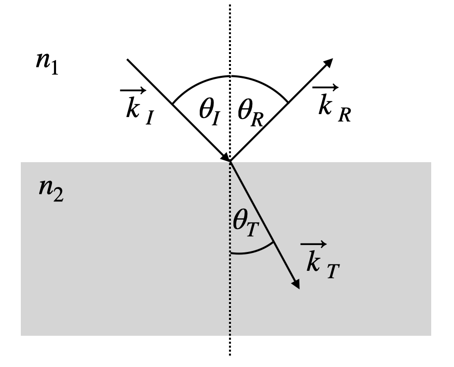
Figure 3— Reflection and refraction at an interface between materials with refractive indices \(n_1\) and \(n_2\).
We have three waves:
Incident: \(\vec{E}_I e^{i(\omega t -\vec{k}_I\cdot \vec{r})}\)
Reflected: \(\vec{E}_R e^{i(\omega t -\vec{k}_R\cdot \vec{r})}\)
Transmitted: \(\vec{E}_T e^{i(\omega t -\vec{k}_T\cdot \vec{r})}\)
Boundary Conditions: The Physics Behind the Rules
The behavior at interfaces comes from Maxwell’s equations. The key boundary conditions are:
Fresnel Equations: Quantifying Reflection and Transmission
The boundary conditions lead to the Fresnel equations, which tell us exactly how much light is reflected and transmitted at interfaces between different media. These equations are derived by applying the boundary conditions that electric and magnetic fields must satisfy at the interface.
To derive the Fresnel equations, we need to consider the polarization of the incident light relative to the plane of incidence (the plane containing the incident ray and the surface normal). There are two fundamental polarization cases:
s-polarization (TE or transverse electric): Electric field is perpendicular to the plane of incidence
p-polarization (TM or transverse magnetic): Electric field is parallel to the plane of incidence
Derivation of Fresnel Equations
For s-polarized light, the electric field is perpendicular to the plane of incidence. Applying the boundary condition that the tangential component of the electric field must be continuous:
\[E_i + E_r = E_t\]
And from the boundary condition for the tangential component of the magnetic field:
For non-magnetic media (\(\mu_1 = \mu_2 = \mu_0\)) and recognizing that \(k_i = k_r\) and \(\theta_i = \theta_r\), and using \(k = \frac{\omega n}{c}\):
These four equations—the reflection and transmission coefficients for both s and p polarizations—are collectively known as the Fresnel equations. They completely describe the behavior of light at an interface between two isotropic media.
The reflected and transmitted intensities (the observable quantities in experiments) can be calculated as:
The factors in the transmission coefficients account for the change in propagation speed and beam cross-section when light crosses the boundary. Energy conservation requires that \(R + T = 1\) for a non-absorbing medium.
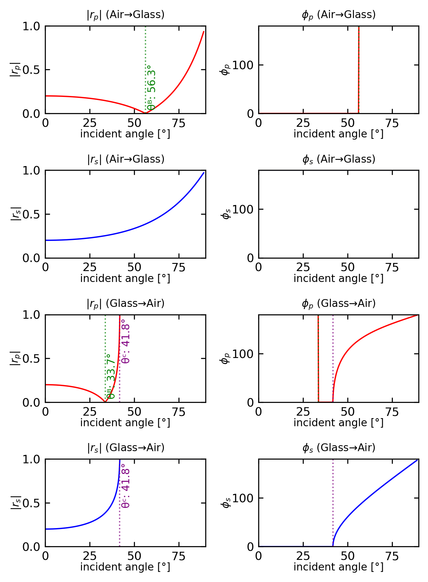
Figure 4— Magnitude and phase of Fresnel reflection coefficients for air-glass and glass-air interfaces. θᴮ marks the Brewster angle where r_p=0, and θᶜ marks the critical angle where total internal reflection begins.
The following code calculates these coefficients for various angles of incidence:
Key Features of Fresnel Behavior
The Fresnel equations reveal several important phenomena that are central to optical systems and devices.
Normal Incidence
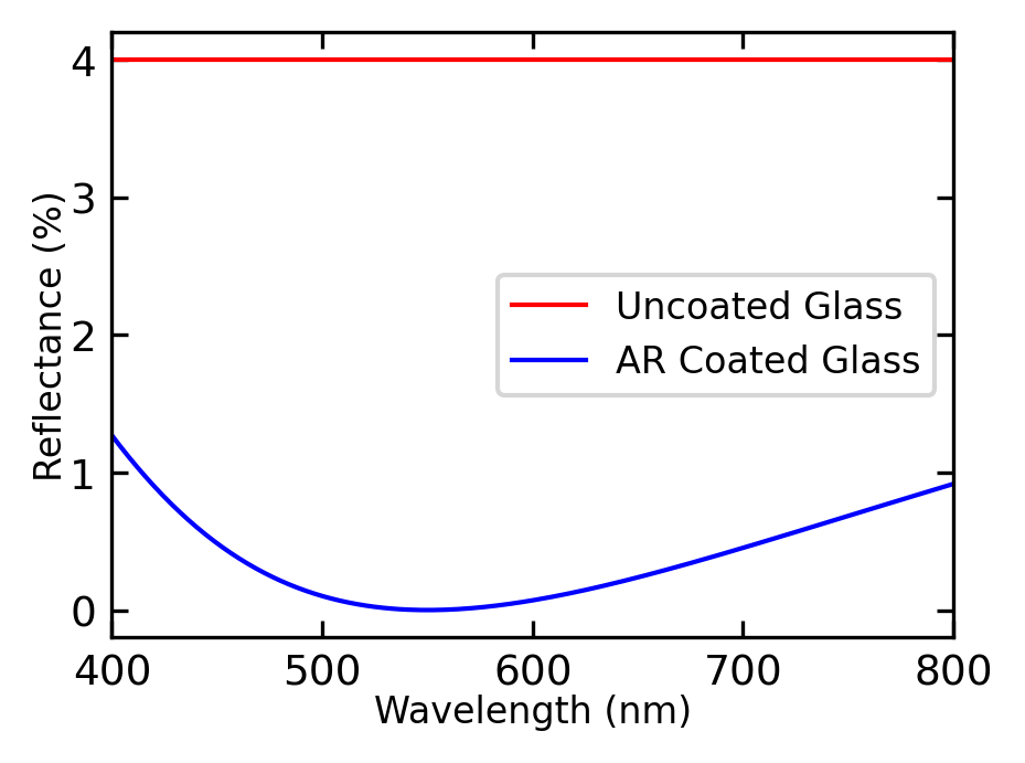
At normal incidence (\(\theta_i = 0\)), both s and p polarization cases become identical, and the reflection coefficient simplifies to:
\[r = \frac{n_1 - n_2}{n_1 + n_2}\]
For an air-glass interface (\(n_1 = 1.0\), \(n_2 = 1.5\)), this gives a reflection of about 4% of the incident intensity. This is why untreated glass reflects approximately 4% of light at each air-glass interface, an important consideration in optical systems like cameras and microscopes where multiple optical elements are used. The intensity loss through a thick glass window with two interfaces would be approximately 8%, which can be significant for precision measurements or energy-sensitive applications.
Brewster’s Angle
A particularly interesting case occurs for p-polarized light at a specific angle called the Brewster angle, given by:
At this angle, the reflection coefficient \(r_p\) becomes exactly zero, meaning p-polarized light is completely transmitted with no reflection. Physically, this occurs because the reflected and refracted rays would be perpendicular to each other, and since light cannot radiate along the direction of the dipole oscillation, no reflection occurs. This property is utilized in:
Polarizing filters (Brewster windows)
Laser systems to minimize internal reflections
Optical systems where polarization control is important
Surface analysis techniques like Brewster angle microscopy
Total Internal Reflection
When light travels from a higher index material to a lower index one (\(n_1 > n_2\)), another important phenomenon occurs. If the angle of incidence exceeds a critical angle:
Snell’s law would require \(\sin\theta_t > 1\), which is physically impossible. Instead, all light is reflected back into the first medium with 100% efficiency, a phenomenon known as total internal reflection (TIR).
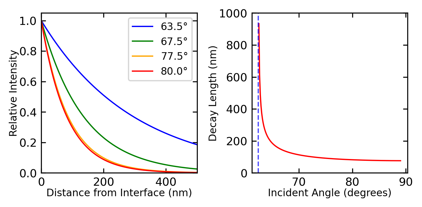
During TIR, an evanescent wave penetrates a short distance (typically a fraction of a wavelength) into the second medium. This wave carries no energy in the perpendicular direction but creates an electromagnetic field that decays exponentially with distance from the interface:
This evanescent field is the basis for techniques like:
Optical waveguides and fibers
Attenuated total reflection (ATR) spectroscopy
Total internal reflection fluorescence (TIRF) microscopy
Fiber optic sensors and evanescent wave coupling devices
Code
# Parameters for TIRFn1 =1.5# Glassn2 =1.33# Watercritical_angle = np.degrees(np.arcsin(n2/n1))wavelength =500# nm in vacuum# Calculate decay length vs. angleangles = np.linspace(critical_angle+0.1, 89, 200) # Range of angles above critical angledecay_lengths = []for angle in angles: theta_rad = np.radians(angle) sin_theta = np.sin(theta_rad) decay = wavelength/(4*np.pi*np.sqrt((n1*sin_theta/n2)**2-1)) decay_lengths.append(decay)# Create figure with two subplotsfig, (ax1, ax2) = plt.subplots(1, 2, figsize=get_size(12, 6))# Plot 1: Field intensity decay from surfacez_values = np.linspace(0, 500, 200) # Distance from surface (nm)selected_angles = [critical_angle+1, critical_angle+5, critical_angle+15, 80]colors = ['blue', 'green', 'orange', 'red']labels = []for i, angle inenumerate(selected_angles):# Calculate decay length for this angle theta_rad = np.radians(angle) sin_theta = np.sin(theta_rad) decay_length = wavelength/(4*np.pi*np.sqrt((n1*sin_theta/n2)**2-1))# Calculate intensity vs distance intensity = np.exp(-z_values/decay_length)# Plot the decay curve ax1.plot(z_values, intensity, color=colors[i], label=f'{angle:.1f}°')ax1.set_xlabel('Distance from Interface (nm)')ax1.set_ylabel('Relative Intensity')ax1.legend()ax1.set_ylim(0, 1.05)ax1.set_xlim(0, 500)# Plot 2: Decay length vs angle (original plot)ax2.plot(angles, decay_lengths, 'r-')ax2.set_xlabel('Incident Angle (degrees)')ax2.set_ylabel('Decay Length (nm)')# Add reference line for critical angleax2.axvline(critical_angle, color='blue', linestyle='--', alpha=0.7)ax2.set_ylim(0, 1000)plt.tight_layout()plt.show()
Figure 5— Evanescent wave characteristics in TIRF microscopy
Experimental Applications and Phenomena
1. Brewster Angle Microscopy (BAM)
At the Brewster angle, p-polarized light experiences zero reflection from a clean interface. Any surface contamination changes this condition, enabling sensitive detection of monolayers.
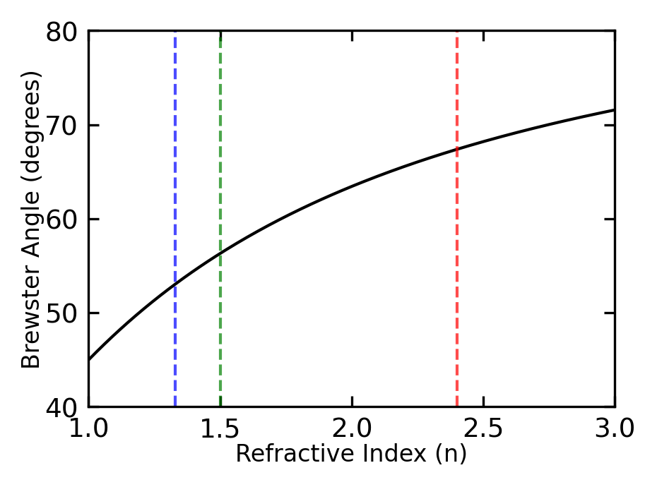
# Define range of refractive indicesn_values = np.linspace(1.0, 3.0, 200)# Calculate Brewster angle (air to medium)brewster_angles = np.degrees(np.arctan(n_values))# Material reference pointsmaterials = [ ('Water', 1.33, 'blue'), ('Glass', 1.5, 'green'), ('Diamond', 2.4, 'red')]fig, ax = plt.subplots(figsize=get_size(8,6))# Plot Brewster angle as function of refractive indexax.plot(n_values, brewster_angles, 'k-', label='Brewster Angle')# Add vertical lines for specific materialsfor name, n, color in materials: angle = np.degrees(np.arctan(n)) ax.axvline(n, color=color, linestyle='--', alpha=0.7)ax.set_xlabel('Refractive Index (n)')ax.set_ylabel('Brewster Angle (degrees)')ax.set_xlim(1.0, 3.0)ax.set_ylim(40, 80)plt.tight_layout()plt.show()
Figure 6— Brewster angle as a function of refractive index for air-medium interfaces. Vertical dashed lines mark specific materials: Water (blue, \(n=1.33\), \(\theta_B=53.1^{°}\)), Glass (green, \(n=1.5\), \(\theta_B=56.3^{°}\)), and Diamond (red, \(n=2.4\), \(\theta_B=67.4^{°}\)).
2. Total Internal Reflection Fluorescence (TIRF) Microscopy
When total internal reflection occurs (\(n_1 > n_2\) and \(\sin\theta_i > n_2/n_1\)), the transmission angle becomes complex:
In this case, the reflection coefficients become complex with unit magnitude (\(|r|^2 = 1\)), meaning 100% of the light is reflected but with a phase shift. This phase shift depends on polarization and is the basis for many optical devices and phenomena.
When light undergoes total internal reflection, an evanescent wave penetrates into the second medium. This wave’s intensity decays exponentially with distance from the interface according to:
\[I(z) = I_0 e^{-z/d}\]
Where the characteristic decay length \(d\) is given by: