In classical optics, light is treated as an electromagnetic wave. However, at the quantum level, light consists of discrete energy packets called photons. The statistical distribution of these photons provides profound insights into the nature of light sources.
The concept of photons, or light quanta, emerged at the dawn of the 20th century, challenging the established wave theory of light. In 1905, Albert Einstein proposed the revolutionary idea that light consists of discrete energy packets (later called photons) to explain the photoelectric effect, building upon Max Planck’s quantum hypothesis of 1900. Einstein’s explanation, which earned him the Nobel Prize in Physics in 1921, was initially met with skepticism from many physicists, including Niels Bohr. Experimental confirmation came gradually, with Robert Millikan’s precise measurements of the photoelectric effect (1916) and Arthur Compton’s demonstration of the particle-like behavior of X-rays (1923). The term “photon” itself was coined by chemist Gilbert Lewis in 1926. By the 1930s, with the development of quantum mechanics, the dual wave-particle nature of light became accepted as fundamental to our understanding of electromagnetic radiation. Today, the photon concept serves as the cornerstone of quantum optics, allowing us to analyze the statistical properties of light with unprecedented precision.
Fundamental Equations for Photon Streams
Before diving into statistical properties, let’s establish some fundamental relationships between classical light intensity and photon descriptions.
The energy of a single photon is related to its frequency by:
\[E_{\text{photon}} = h\nu = \frac{hc}{\lambda}\]
where \(h\) is Planck’s constant, \(\nu\) is the frequency, \(c\) is the speed of light, and \(\lambda\) is the wavelength.
For a classical electromagnetic wave with intensity \(I\) (power per unit area), the corresponding photon flux \(\Phi\) (number of photons per unit area per unit time) is:
\[\Phi = \frac{I}{h\nu}\]
The total number of photons \(n\) passing through an area \(A\) during time \(T\) is:
\[n = \Phi \cdot A \cdot T = \frac{I \cdot A \cdot T}{h\nu}\]
For a detector with quantum efficiency \(\eta\) (the probability that an incident photon generates a detectable event), the average number of detected photons becomes:
\[\bar{n} = \eta \cdot n = \eta \cdot \frac{I \cdot A \cdot T}{h\nu}\]
The photon arrival rate \(\alpha\) (photons per unit time) can be expressed as:
This photon arrival rate \(\alpha\) is a crucial parameter that connects the classical description of light intensity with the quantum description of photon statistics that we’ll explore in the following sections.
Random Photon Streams and Poisson Statistics
Photon Streams and Time Bins
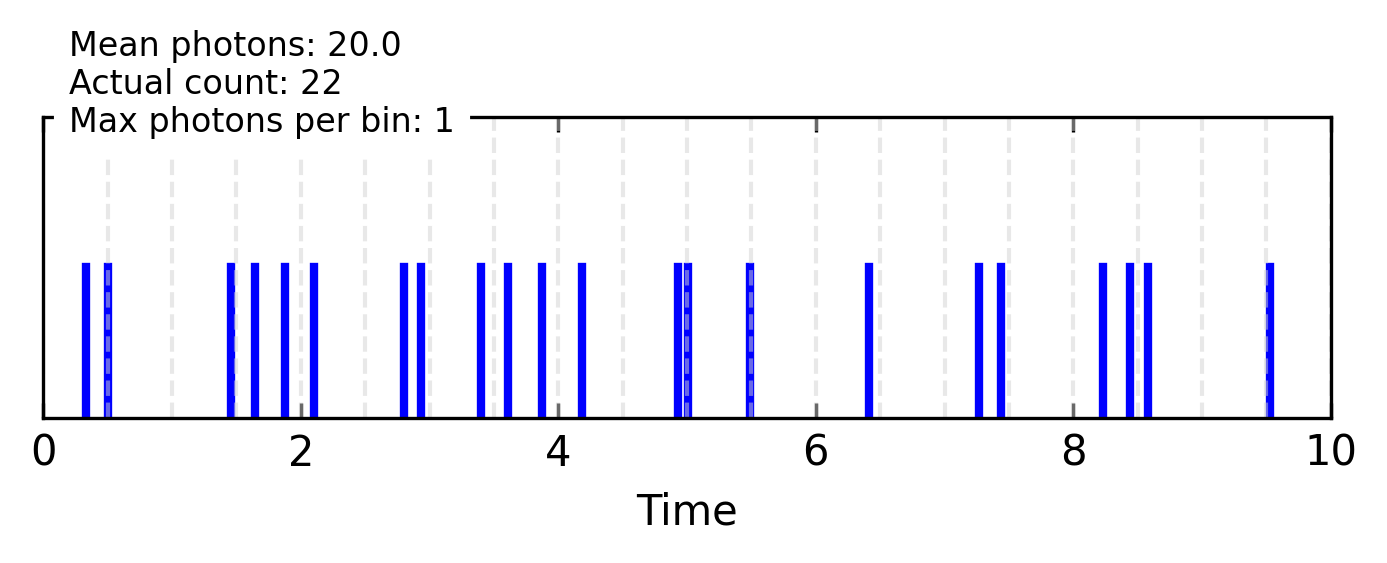
To understand photon statistics, we first need to conceptualize light as a stream of discrete photons arriving at a detector over time. Let’s develop a model where we divide our total observation time \(T\) into \(M\) equal time bins, each of duration \(\Delta t = T/M\).
For a light source with average intensity \(I\), the average number of photons expected in the entire observation period is \(\bar{n} = \alpha T\), where \(\alpha\) is proportional to the intensity. The average number of photons per time bin is therefore \(\mu = \bar{n}/M = \alpha \Delta t\).
In a random photon stream, the arrival of each photon is an independent event with no memory of previous arrivals. This means that for small enough time bins, each bin has: - A probability \(p = \mu\) of containing exactly one photon - A probability \(1-p\) of containing no photons - A negligible probability of containing more than one photon (for sufficiently small \(\Delta t\))
Code
# Generate a random photon streamnp.random.seed(42) # For reproducibilitytotal_time =10# Total observation time Tnum_bins =200# Increased number of time bins M to ensure at most 1 photon per bindt = total_time / num_bins # Width of each time bin# Average photon rate (mean photons per unit time)photon_rate =2# Reduced alpha in the notes to ensure fewer photonsmean_photons = photon_rate * total_time # Total mean photon number over time Tmu = mean_photons / num_bins # Probability of photon per bin# Generate random photons based on probability mu for each bin# Ensuring at most one photon per binphoton_events = np.random.random(num_bins) < mu# Generate random positions within each bin for the photonsphoton_times = []for bin_idx in np.where(photon_events)[0]:# Place photon randomly within its bin, not at the edge rand_position = bin_idx * dt + np.random.random() * dt photon_times.append(rand_position)photon_times = np.array(photon_times)# Verify no bin has more than one photonbin_counts = np.histogram(photon_times, bins=num_bins, range=(0, total_time))[0]max_photons_per_bin = np.max(bin_counts)# Create the figurefig, ax = plt.subplots(figsize=get_size(12, 5))# Plot vertical lines for each photonfor t in photon_times: ax.plot([t, t], [0, 1], 'b-', linewidth=2)# Add grid lines to show time binsfor i inrange(num_bins +1):if i %10==0: # Only show every 10th grid line to avoid clutter ax.axvline(i * dt, color='lightgray', linestyle='--', alpha=0.5)# Set axis limits and labelsax.set_xlim(0, total_time)ax.set_ylim(0, 2)ax.set_yticks([])ax.set_xlabel('Time')# Add text showing statisticsactual_count =len(photon_times)ax.text(0.02, 0.95,f"Mean photons: {mean_photons:.1f}\nActual count: {actual_count}\nMax photons per bin: {max_photons_per_bin}", transform=ax.transAxes, backgroundcolor='white', fontsize=8)plt.tight_layout()plt.show()
Figure 1— Random photon stream showing individual photons (vertical lines) arriving at random times. The time axis is divided into bins of width \(\Delta t\). Each bin contains either 0 or 1 photons in this simplified model, with the probability of finding a photon in any given bin being equal to \(\mu = \bar{n}/M\).
From Time Bins to Binomial Distribution
Given these properties, we can calculate the probability \(P(n,M)\) of detecting exactly \(n\) photons in \(M\) time bins. This is equivalent to asking: what is the probability of having exactly \(n\) successes in \(M\) independent trials, where the probability of success in each trial is \(p = \mu\)?
where \(\binom{M}{n} = \frac{M!}{n!(M-n)!}\) is the binomial coefficient representing the number of ways to choose \(n\) time bins from \(M\) total bins.
The Poisson Limit
Now, let’s consider what happens as we make our time bins smaller and more numerous. In the limit where \(M \to \infty\) and \(\Delta t \to 0\), while keeping the total observation time \(T\) and the average photon number \(\bar{n}\) constant:
The number of bins \(M\) increases
The probability per bin \(\mu = \bar{n}/M\) decreases
The product \(M\mu = \bar{n}\) remains constant
In this limit, the binomial distribution approaches the Poisson distribution. To see this, we substitute \(\mu = \bar{n}/M\) into the binomial formula:
where \(\bar{n}\) is the mean photon number in the interval.
Properties of the Poisson Distribution
The Poisson distribution has the remarkable property that its variance equals its mean:
\[\langle (\Delta n)^2 \rangle = \langle n \rangle = \bar{n}\]
This equal mean and variance is a signature of the randomness in the photon arrival process, where events occur independently and at a constant average rate.
To verify this property, we can calculate the mean and variance directly from the probability distribution:
The mean: \(\langle n \rangle = \sum_{n=0}^{\infty} n P(n) = \bar{n}\)
The signal-to-noise ratio (SNR) is a crucial metric in experimental physics, quantifying our ability to distinguish a signal from the background noise. For a measurement, the SNR is defined as the ratio of the mean signal to the standard deviation of the noise:
\[\text{SNR} = \frac{\text{signal}}{\text{noise}} = \frac{\langle n \rangle}{\sqrt{\langle (\Delta n)^2 \rangle}}\]
For random light following Poisson statistics, we have:
This relationship reveals an important property of random light: the SNR scales as the square root of the mean photon number. This is known as the “shot noise limit” and represents a fundamental quantum limit to measurement precision with coherent light. To improve the SNR by a factor of 2, we need to increase the light intensity (or integration time) by a factor of 4.
This \(\sqrt{\bar{n}}\) scaling of SNR is a direct consequence of the statistical independence of photon arrivals in coherent light and plays a crucial role in determining the sensitivity limits of optical measurements, from astronomical observations to laser-based communications.
This statistical behavior is characteristic of coherent light sources such as ideal lasers, where photon emission events are independent of each other.
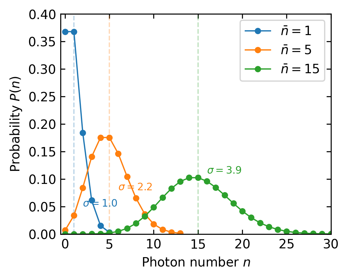
Figure 2— Poisson distribution of photon number statistics for three different mean photon numbers. The plot shows the probability \(P(n)\) of detecting exactly \(n\) photons for light with mean photon number \(\bar{n}\). As the mean increases, the distribution broadens with variance equal to the mean, demonstrating the characteristic \(\sqrt{\bar{n}}\) fluctuations of coherent light.
Beam Splitters and Photon Statistics
A beam splitter is an optical component that splits an incident beam into two parts. For a 50:50 beam splitter, an incoming photon has equal probability of being transmitted or reflected. Interestingly, when random (Poissonian) light is incident on a beam splitter, the statistics of the output beams remain Poissonian.
To understand why, consider that each photon in the input beam makes an independent decision to be transmitted or reflected. If the input beam has Poisson statistics with mean \(\bar{n}\), the transmitted beam will have a mean of \(\bar{n}_T = R\bar{n}\) and the reflected beam will have a mean of \(\bar{n}_R = T\bar{n}\), where \(R\) and \(T\) are the reflection and transmission coefficients (\(R + T = 1\)).
The independence of photon behavior ensures that both output beams maintain Poisson statistics, just with scaled means. This is mathematically represented as:
This preservation of statistics is a direct consequence of the binomial sampling of the original Poisson distribution, which yields another Poisson distribution.
Thermal Light and Exponential Statistics
Thermal light, such as that emitted by incandescent bulbs or stars, exhibits different statistical properties. The emission process in thermal sources involves atoms transitioning between energy levels due to thermal excitation. This process leads to what we call “bunching” of photons.
For thermal light, the probability distribution of photons follows:
\[P(n) = \frac{\bar{n}^n}{(1+\bar{n})^{n+1}}\]
This distribution results in a variance that exceeds the mean:
\[\langle (\Delta n)^2 \rangle = \langle n \rangle + \langle n \rangle^2 = \bar{n} + \bar{n}^2\]
The photon number fluctuations are larger than in coherent light, reflecting the bunching tendency of thermal photons. This bunching arises from the Bose-Einstein statistics governing photons, which encourages multiple photons to occupy the same mode.
The intensity fluctuations of thermal light follow an exponential distribution:
\[P(I) = \frac{1}{\langle I \rangle} e^{-I/\langle I \rangle}\]
This exponential behavior is a direct consequence of the random nature of thermal emission processes, where the radiation field is built up from the contributions of many independent atomic emitters.
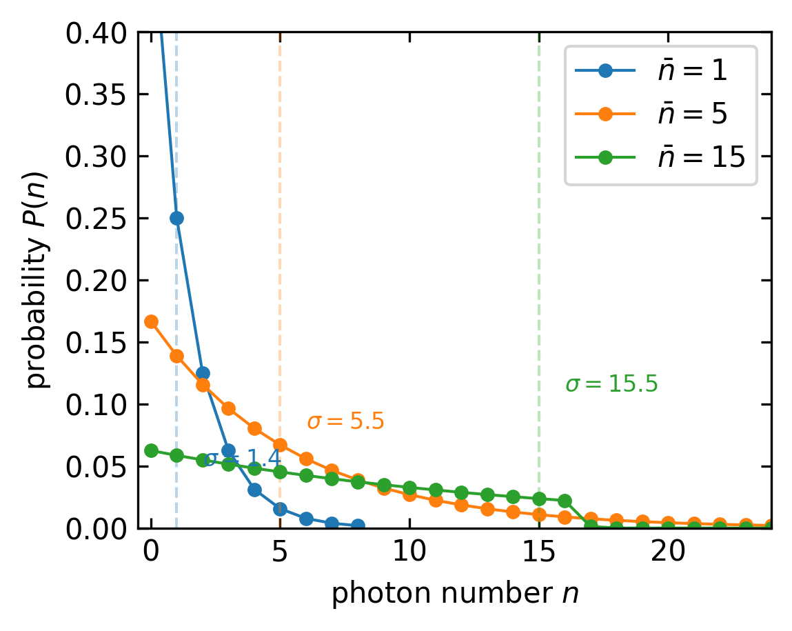
Figure 3— Thermal light distribution of photon number statistics for three different mean photon numbers. The plot shows the probability \(P(n)\) of detecting exactly \(n\) photons for thermal light with mean photon number \(\bar{n}\). Compared to the Poisson distribution, thermal light shows more significant photon bunching, with higher probabilities for both zero photons and large photon numbers, demonstrating the characteristic excess noise proportional to \(\bar{n}^2\).
Signal-to-Noise Ratio for Thermal Light
The signal-to-noise ratio for thermal light differs significantly from that of coherent light due to the different statistical distribution of photons. Using the definition of SNR as the ratio of mean signal to the standard deviation of noise:
\[\text{SNR} = \frac{\langle n \rangle}{\sqrt{\langle (\Delta n)^2 \rangle}}\]
For thermal light, with \(\langle (\Delta n)^2 \rangle = \bar{n} + \bar{n}^2\), we have:
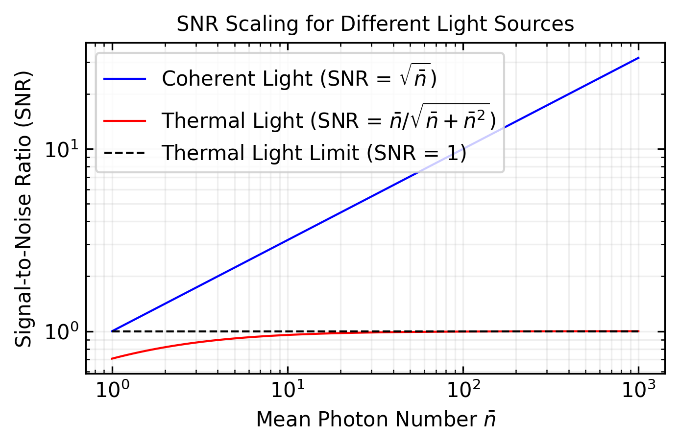
This is a striking result: for thermal light at high intensities, the SNR approaches a constant value of 1, regardless of how much we increase the intensity. This is in stark contrast to the coherent light case where SNR increases as \(\sqrt{\bar{n}}\).
This fundamental limitation on the SNR of thermal light is due to the inherent “excess noise” from photon bunching. It explains why many precision optical measurements preferentially use laser sources (with Poisson statistics) rather than thermal sources, even when high intensities are available.
The comparison between thermal light (SNR ~ 1) and coherent light (SNR ~ \(\sqrt{\bar{n}}\)) provides a clear example of how the quantum statistical properties of a light source directly impact measurement sensitivity in practical applications.
Code
# Range of mean photon numbers mean_values = np.logspace(0, 3, 100)# Calculate SNR for coherent (Poisson) light snr_coherent = np.sqrt(mean_values)# Calculate SNR for thermal light snr_thermal = mean_values / np.sqrt(mean_values + mean_values**2) plt.figure(figsize=get_size(12,8)) plt.loglog(mean_values, snr_coherent, 'b-', label='Coherent Light (SNR = $\\sqrt{\\bar{n}}$)') plt.loglog(mean_values, snr_thermal, 'r-', label='Thermal Light (SNR = $\\bar{n}/\\sqrt{\\bar{n}+\\bar{n}^2}$)') plt.loglog(mean_values, np.ones_like(mean_values), 'k--', label='Thermal Light Limit (SNR = 1)') plt.xlabel('Mean Photon Number $\\bar{n}$') plt.ylabel('Signal-to-Noise Ratio (SNR)') plt.title('SNR Scaling for Different Light Sources') plt.grid(True, which="both", ls="-", alpha=0.2) plt.legend() plt.tight_layout() plt.show()