Introduction to Gaussian Beams
In optics and laser physics, Gaussian beams represent one of the most fundamental and important mathematical descriptions of laser light propagation. They are particularly relevant for understanding laser resonators, optical systems, and coherent light behavior. This section introduces Gaussian beams from first principles and explores their mathematical description.
Derivation from the Helmholtz Equation
We begin with the Helmholtz equation, which describes monochromatic electromagnetic waves in a homogeneous medium:
\[\nabla^2 U + k^2 U = 0\]
where \(U\) represents the electric field component, \(k = 2\pi/\lambda\) is the wave number, and \(\lambda\) is the wavelength of light. For a wave predominantly traveling along the \(z\)-axis, we can express the electric field as:
\[U(x,y,z) = u(x,y,z)e^{-ikz}\]
Here, \(u(x,y,z)\) is a complex amplitude function that varies slowly with \(z\) compared to the wavelength. Substituting this into the Helmholtz equation and expanding the Laplacian operator yields:
\[\left(\frac{\partial^2}{\partial x^2} + \frac{\partial^2}{\partial y^2} + \frac{\partial^2}{\partial z^2}\right)(u e^{-ikz}) + k^2 (u e^{-ikz}) = 0\]
Computing the derivatives and simplifying:
\[\frac{\partial^2 u}{\partial x^2} + \frac{\partial^2 u}{\partial y^2} + \frac{\partial^2 u}{\partial z^2} - 2ik\frac{\partial u}{\partial z} = 0\]
The Paraxial Approximation
The paraxial approximation applies when the beam’s angular spread is small, meaning the wavefronts are nearly perpendicular to the propagation axis. Mathematically, this means that the amplitude \(u\) varies slowly along the propagation direction compared to transverse directions:
\[\left|\frac{\partial^2 u}{\partial z^2}\right| \ll \left|2k\frac{\partial u}{\partial z}\right|\]
Under this approximation, the Helmholtz equation simplifies to the paraxial Helmholtz equation:
\[\frac{\partial^2 u}{\partial x^2} + \frac{\partial^2 u}{\partial y^2} - 2ik\frac{\partial u}{\partial z} = 0\]
To solve this equation, we propose the ansatz:
\[u(x,y,z) = A(z)\exp\left[-\frac{k}{2q(z)}(x^2 + y^2)\right]\]
where \(A(z)\) and \(q(z)\) are complex functions to be determined. Substituting this into the paraxial equation and solving the resulting differential equations:
\[\frac{dq}{dz} = 1 \quad \text{and} \quad \frac{dA}{dz} = -\frac{A}{q}\]
These yield solutions \(q(z) = q_0 + z\) and \(A(z) = \frac{A_0}{q(z)}\), where \(q_0\) and \(A_0\) are constants.
The complex beam parameter \(q(z)\) relates to physical parameters through:
\[\frac{1}{q(z)} = \frac{1}{R(z)} - i\frac{\lambda}{\pi w^2(z)}\]
where \(R(z)\) is the radius of curvature of the wavefront and \(w(z)\) is the beam radius at which the intensity falls to \(1/e^2\) of its axial value.
Setting \(q_0 = iz_0\) where \(z_0\) is the Rayleigh range, we can express these parameters as:
\[w(z) = w_0\sqrt{1 + \left(\frac{z}{z_0}\right)^2}\]
\[R(z) = z\left[1 + \left(\frac{z_0}{z}\right)^2\right]\]
where \(w_0 = \sqrt{\frac{\lambda z_0}{\pi}}\) is the beam waist (minimum beam radius).
The complete Gaussian beam solution is:
\[U(x,y,z) = U_0 \frac{w_0}{w(z)} \exp\left[-\frac{x^2 + y^2}{w^2(z)}\right] \exp\left[-ikz - ik\frac{x^2 + y^2}{2R(z)} + i\phi(z)\right]\]
where \(\phi(z) = \arctan(z/z_0)\) is the Gouy phase shift, representing an additional phase beyond that of a plane wave.
In scalar wave theory, the intensity of the Gaussian beam is proportional to the square of the amplitude. It can be calculated as:
\[I(x,y,z) = |U(x,y,z)|^2 = I_0\frac{w_0^2}{w^2(z)}\exp\left[-\frac{2(x^2+y^2)}{w^2(z)}\right]\]
where \(I_0 = |U_0|^2\) is the peak intensity at the beam waist. This expression shows that the intensity has a Gaussian profile in any transverse plane, with its peak on the beam axis. The intensity falls to \(1/e^2\) of its axial value at a radial distance \(r = w(z)\) from the axis, which defines the beam radius. The total power carried by the beam is conserved during propagation, but the peak intensity decreases as \(w(z)\) increases with distance from the waist.
Gaussian Beam Propagation in the x-z Plane
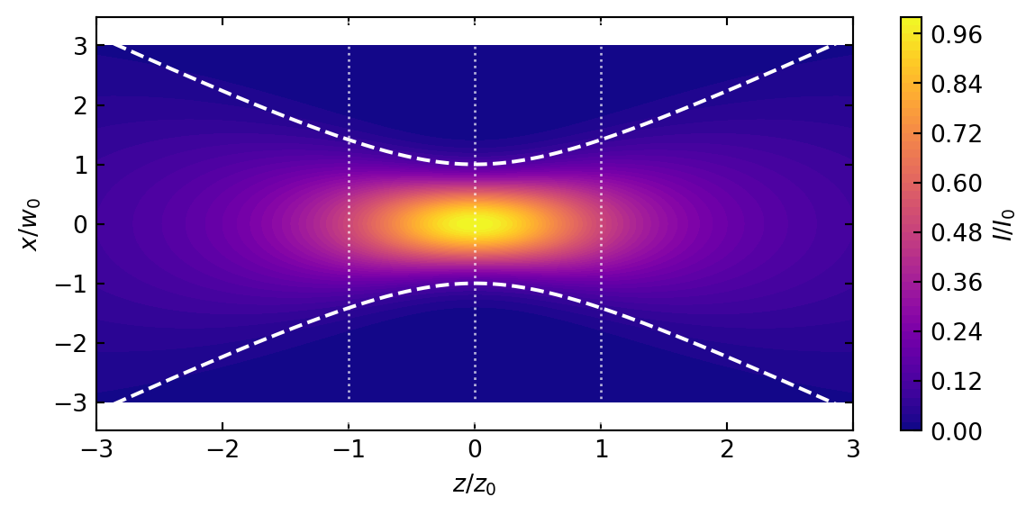
We can visualize how a Gaussian beam’s intensity varies across both the propagation direction (z-axis) and transverse direction (x-axis) simultaneously using a 2D contour plot.
This contour plot illustrates how the Gaussian beam intensity distribution evolves as it propagates. The horizontal axis represents the normalized propagation distance (\(z/z_0\)), while the vertical axis shows the normalized transverse distance (\(x/w_0\)). The color gradient indicates intensity values, with brighter colors representing higher intensities.
The white dashed lines trace the beam width \(w(z)\), where the intensity falls to \(1/e^2\) (approximately 13.5%) of its value on the beam axis. Note how the beam width reaches its minimum at the beam waist (\(z=0\)) and expands as the beam propagates away from the focus.
The plot clearly shows that the highest intensity occurs at the beam waist, with the intensity decreasing both as we move away from the center axis and as the beam propagates away from the focal point.
Key Gaussian Beam Parameters
The following table summarizes the important parameters that characterize a Gaussian beam:
| Parameter | Expression | Description |
|---|---|---|
| Beam waist (\(w_0\)) | Minimum beam radius at focus (\(z=0\)) | |
| Beam width (\(w(z)\)) | \(w(z) = w_0\sqrt{1 + \left(\frac{z}{z_0}\right)^2}\) | Beam radius at position \(z\) |
| Rayleigh length (\(z_0\)) | \(z_0 = \frac{\pi w_0^2}{\lambda}\) | Distance over which beam area doubles |
| Radius of curvature (\(R(z)\)) | \(R(z) = z\left[1 + \left(\frac{z_0}{z}\right)^2\right]\) | Radius of wavefront curvature |
| Divergence angle (\(\theta\)) | \(\theta = \frac{\lambda}{\pi w_0}\) | Far-field half-angle of beam spread |
| Gouy phase (\(\phi(z)\)) | \(\phi(z) = \arctan\left(\frac{z}{z_0}\right)\) | Additional phase beyond plane wave |
| Complex beam parameter (\(q(z)\)) | \(q(z) = z + iz_0\) | Combined parameter for beam properties |
These parameters are interrelated, forming a complete description of how a Gaussian beam propagates. The Rayleigh length \(z_0\) is particularly important as it defines the transition between the near field (where the beam is approximately collimated) and the far field (where the beam diverges linearly). At a distance of one Rayleigh length from the waist, the beam width increases by a factor of \(\sqrt{2}\) and the intensity drops to half its maximum value.
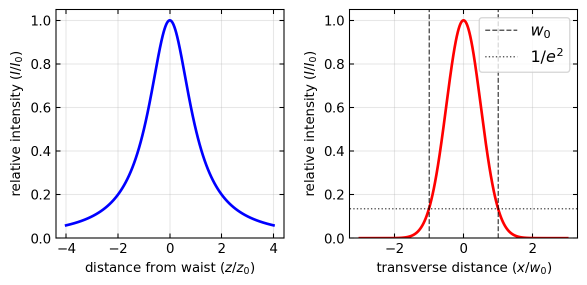
Gaussian Beam Intensity Profiles
To better understand the spatial distribution of intensity in a Gaussian beam, it’s helpful to visualize how the intensity varies along different directions. Here we explore two fundamental cross-sections: the axial intensity along the beam propagation path, and the transverse intensity profile at the beam waist.
Gaussian Beam Propagation
To better understand the spatial evolution of a Gaussian beam as it propagates, we can visualize how two key parameters change with distance: the beam width \(w(z)\) and the wavefront radius of curvature \(R(z)\).
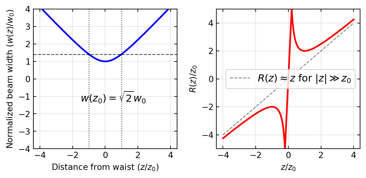
The left plot shows how the beam width \(w(z)\) evolves with distance from the beam waist. At \(z = 0\), the beam is at its narrowest point \(w_0\). At the Rayleigh range (\(z = ±z_0\)), the width increases to \(\sqrt{2}w_0\). For \(|z| \gg z_0\), the beam width increases approximately linearly with distance, corresponding to a constant far-field divergence angle \(\theta = \lambda/(\pi w_0)\).
The right plot illustrates the wavefront radius of curvature \(R(z)\). At the beam waist, the wavefronts are flat (\(R = \infty\)). The curvature reaches its minimum absolute value of \(2z_0\) at \(z = ±z_0\). For \(z > 0\), \(R(z)\) is positive (converging wavefronts), while for \(z < 0\), \(R(z)\) is negative (diverging wavefronts). As \(|z|\) increases, \(R(z)\) approaches the asymptotic behavior of a spherical wave, where \(R(z) \approx z\).
These parameters together provide a complete description of how the Gaussian beam transforms from a tightly focused wave near the waist to an approximately spherical wave in the far field.
Gaussian Beam Transformation Through Optical Systems
The ABCD Matrix Formalism
The propagation of Gaussian beams through optical systems can be elegantly described using the ABCD matrix formalism from ray optics. While ray optics typically tracks the position and angle of rays, for Gaussian beams we track the transformation of the complex beam parameter \(q(z)\).
When a Gaussian beam passes through an optical system characterized by an ABCD matrix, the complex beam parameter transforms according to:
\[q_2 = \frac{Aq_1 + B}{Cq_1 + D}\]
where \(q_1\) is the initial complex beam parameter and \(q_2\) is the transformed parameter. This remarkable result, known as the ABCD law for Gaussian beams, allows us to determine how the beam waist and wavefront curvature change through arbitrary optical systems.
Common Optical Elements
Different optical elements transform Gaussian beams in characteristic ways:
Free-space propagation over distance \(d\) is represented by:
\[\begin{pmatrix} A & B \\ C & D \end{pmatrix} = \begin{pmatrix} 1 & d \\ 0 & 1 \end{pmatrix}\]
This matrix describes how the beam naturally diverges as it propagates.
Thin lens with focal length \(f\):
\[\begin{pmatrix} A & B \\ C & D \end{pmatrix} = \begin{pmatrix} 1 & 0 \\ -1/f & 1 \end{pmatrix}\]
A lens modifies the wavefront curvature without changing the beam diameter at the lens location.
Curved interface between media with refractive indices \(n_1\) and \(n_2\) and radius of curvature \(R\):
\[\begin{pmatrix} A & B \\ C & D \end{pmatrix} = \begin{pmatrix} 1 & 0 \\ -\frac{n_2-n_1}{n_2 R} & \frac{n_1}{n_2} \end{pmatrix}\]
Multiple optical elements can be analyzed by multiplying their respective ABCD matrices in the order encountered by the beam.
Focusing of Gaussian Beams
Consider a Gaussian beam whose waist \(w_0\) lies at the lens plane (i.e., the wavefront is flat at the lens, \(R\to\infty\)). The complex beam parameter at the lens is \(q = iz_R\) with \(z_R = \pi w_0^2/\lambda\). Applying the thin-lens ABCD matrix transforms the parameter as:
\[\frac{1}{q'} = \frac{1}{q} - \frac{1}{f} = -\frac{1}{f} - \frac{i}{z_R}\]
Propagating \(q'\) a distance \(d\) and requiring the wavefront to be flat (Re\((1/q'(d)) = 0\)) gives the exact position and size of the new waist:
\[d' = \frac{f\,z_R^2}{z_R^2 + f^2}, \qquad \boxed{w_0' = \frac{f\,w_0}{\sqrt{z_R^2 + f^2}}}\]
The new waist is always located at \(d' \leq f\), approaching the focal point only when \(z_R \gg f\).
Paraxial (collimated) approximation. When the input beam is well collimated at the lens (\(z_R \gg f\), i.e., \(\pi w_0^2 \gg \lambda f\)), the exact formula simplifies to:
\[w_0' \approx \frac{f\,w_0}{z_R} = \frac{\lambda f}{\pi w_0}, \qquad d' \approx f\]
This is the result commonly quoted in optics texts. It shows that smaller focal spots require larger input beams: halving \(w_0\) doubles \(w_0'\). The condition \(z_R \gg f\) is easily satisfied for typical laboratory situations (e.g., \(w_0 = 1\,\mathrm{mm}\), \(\lambda = 0.5\,\mu\mathrm{m}\), \(f = 100\,\mathrm{mm}\) gives \(z_R \approx 6\,\mathrm{m} \gg f\)), but breaks down for micro-optics or highly divergent input beams.
The Rayleigh range and divergence angle of the focused beam follow directly:
\[z_0' = \frac{\pi w_0'^2}{\lambda} \approx \frac{\lambda f^2}{\pi w_0^2} = \frac{f^2}{z_R}, \qquad \theta' = \frac{\lambda}{\pi w_0'} \approx \frac{w_0}{f}\]
The divergence angle \(\theta' = w_0/f\) is the geometric half-angle subtended by the input beam at the lens — a direct link between ray optics and the Gaussian beam picture. Tightly focused beams (\(w_0'\) small) inevitably have short Rayleigh ranges and diverge rapidly beyond the focus: the product \(w_0'\,\theta' = \lambda/\pi\) is invariant and sets the fundamental trade-off between spot size and depth of focus.
Higher-Order Gaussian Modes
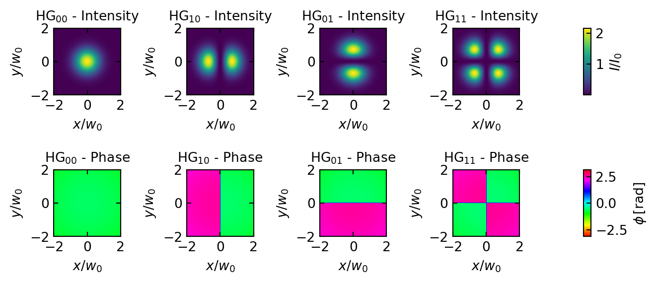
Hermite-Gaussian Beams
Hermite-Gaussian modes form a complete set of solutions to the paraxial wave equation in Cartesian coordinates. They can be expressed as:
\[U_{nm}(x,y,z) = U_0\frac{w_0}{w(z)}H_n\left(\frac{\sqrt{2}x}{w(z)}\right)H_m\left(\frac{\sqrt{2}y}{w(z)}\right) \exp\left[-\frac{x^2 + y^2}{w^2(z)}\right]\] \[\times \exp\left[-ikz - ik\frac{x^2 + y^2}{2R(z)} + i(n+m+1)\phi(z)\right]\]
where \(H_n\) and \(H_m\) are Hermite polynomials of orders \(n\) and \(m\). The indices \(n,m = 0,1,2,...\) determine the number of nodes in the intensity pattern along \(x\) and \(y\) directions. The fundamental Gaussian beam corresponds to \(n=m=0\).
These modes naturally arise in laser resonators with rectangular symmetry and maintain their intensity pattern during propagation, though they scale in size. Each higher-order mode experiences an additional Gouy phase shift, causing different modes to accumulate phase at different rates during propagation.
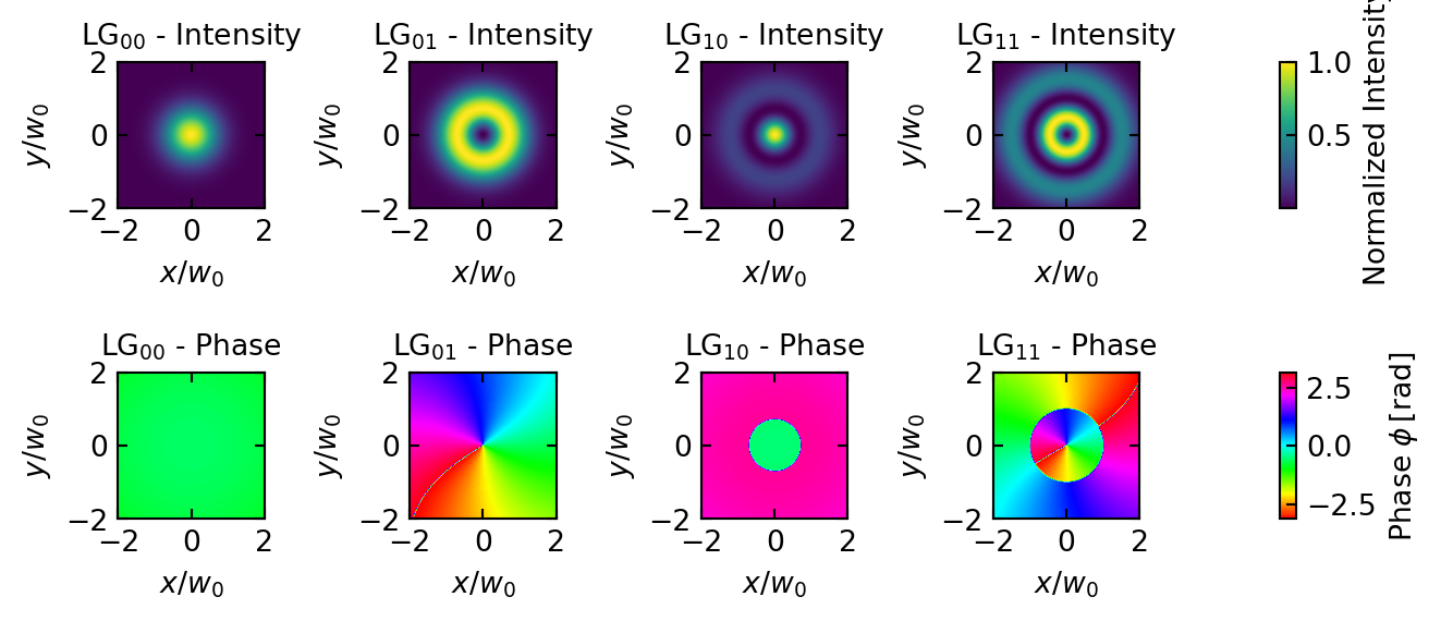
Laguerre-Gaussian Beams
In systems with cylindrical symmetry, Laguerre-Gaussian modes provide a more natural description. In cylindrical coordinates \((r,\theta,z)\), they are given by:
\[U_{pl}(r,\theta,z) = U_0\frac{w_0}{w(z)}\left(\frac{\sqrt{2}r}{w(z)}\right)^{|l|}L_p^{|l|}\left(\frac{2r^2}{w^2(z)}\right) \exp\left[-\frac{r^2}{w^2(z)}\right]\] \[\times \exp\left[-ikz - ik\frac{r^2}{2R(z)} + i(2p+|l|+1)\phi(z) + il\theta\right]\]
where \(L_p^{|l|}\) are the associated Laguerre polynomials, \(p \geq 0\) is the radial index determining the number of radial nodes, and \(l\) is the azimuthal index that determines the helical structure of the wavefront.
A remarkable property of Laguerre-Gaussian modes with \(l \neq 0\) is that they carry orbital angular momentum (OAM) of \(l\hbar\) per photon. This OAM arises from the helical phase structure represented by the term \(\exp(il\theta)\), which creates a twisted wavefront resembling a spiral staircase. The intensity distribution forms a ring-like pattern with a dark center for \(l \neq 0\) due to the phase singularity along the beam axis. As \(p\) increases, additional concentric rings appear in the intensity pattern.
The orbital angular momentum of light is distinct from spin angular momentum (SAM), which is associated with circular polarization (±\(\hbar\) per photon). While SAM relates to the polarization state of light, OAM relates to the spatial structure of the wavefront. Importantly, these two forms of angular momentum can interact through spin-orbit coupling in certain optical systems, particularly in anisotropic or inhomogeneous media, at interfaces, or when light experiences strong focusing. Such spin-orbit coupling enables novel phenomena like spin-to-orbital angular momentum conversion, where the polarization state can influence the spatial structure of the beam and vice versa. This coupling mechanism has found specific applications in:
Optical tweezers - Spin-orbit coupling allows precise control of trapped particles by converting polarization changes into rotational motion, enabling manipulation of microscopic objects with unprecedented precision.
Quantum cryptography - The coupling between SAM and OAM creates additional degrees of freedom for encoding quantum information, enhancing the security and information capacity of quantum key distribution protocols.
Optical vortex metrology - Using the phase singularities created by spin-orbit interactions to detect nanoscale surface imperfections with superior sensitivity compared to conventional techniques.
Chiral spectroscopy - The interaction between polarization and spatial modes enables enhanced detection of chiral molecules by amplifying the difference in light-matter interactions between enantiomers.
Structured light microscopy - Coupling between SAM and OAM generates complex field patterns that improve resolution beyond the diffraction limit in specific imaging configurations.
Both families of higher-order modes are important in modern optics applications, including optical manipulation, quantum information processing, and mode-division multiplexing in optical communications. They represent different orthogonal bases of the same solution space and can be transformed into each other through appropriate optical systems.
Bessel Beams
While Hermite-Gaussian and Laguerre-Gaussian modes emerge as solutions to the paraxial wave equation, Bessel beams are exact solutions of the full Helmholtz equation that possess the remarkable property of being non-diffracting: their transverse intensity profile is invariant under propagation.
Derivation
We seek solutions to the Helmholtz equation in cylindrical coordinates \((r, \varphi, z)\) by separation of variables. Writing \(U(r,\varphi,z) = R(r)\Phi(\varphi)Z(z)\) and separating, the radial part must satisfy Bessel’s differential equation
\[\frac{d^2 R}{dr^2} + \frac{1}{r}\frac{dR}{dr} + \left(k_r^2 - \frac{l^2}{r^2}\right) R = 0,\]
whose bounded solutions are Bessel functions of the first kind \(J_l(k_r r)\). The full ideal Bessel beam of order \(l\) is:
\[U_l(r,\varphi,z) = A_0\, J_l(k_r r)\, e^{il\varphi}\, e^{ik_z z},\]
where the transverse and longitudinal wave-vector components satisfy the constraint \(k_r^2 + k_z^2 = k^2 = (n\omega/c)^2\).
Because the intensity \(I \propto |J_l(k_r r)|^2\) depends only on \(r\), not on \(z\), the transverse profile is truly propagation-invariant. The cone half-angle of the associated conical wavefront is \(\theta_c = \arcsin(k_r/k)\).
Key Properties
| Property | Gaussian beam | Bessel beam |
|---|---|---|
| Diffracts? | Yes (\(w \propto z\)) | No (ideal) |
| Finite energy? | Yes | No (ideal) |
| Orbital angular momentum | Only for LG modes | \(l\hbar\) per photon |
| Self-healing | No | Yes |
| Realisation | Direct from laser | Axicon / annular aperture |
Self-healing is a striking consequence of the conical wave structure: if an obstacle blocks the beam at one transverse location, the interfering plane waves reconstruct the pattern beyond a healing distance \(z_\text{heal} \approx r_\text{obs}/\tan\theta_c\).
Ideal Bessel beams carry infinite power because \(\int_0^\infty J_l^2(k_r r)\,r\,dr\) diverges. In practice, Bessel-Gaussian beams are generated by multiplying by a Gaussian envelope, giving an approximately non-diffracting beam over a finite depth of field \(z_\text{max} \approx w_0/\tan\theta_c\).
Generation with an Axicon
An axicon (conical lens with apex angle \(\alpha\)) converts an incident Gaussian beam into a Bessel-Gaussian beam. A plane wave hitting the axicon acquires a radially linear phase \(\exp(-ik_r r)\) with \(k_r = k(n-1)\alpha\), producing a bright on-axis line focus extending from the lens to \(z_\text{max}\). The on-axis intensity oscillates (interference between the inward-travelling cone and the outward cone) and reaches a peak at \(z_\text{max}/2\).
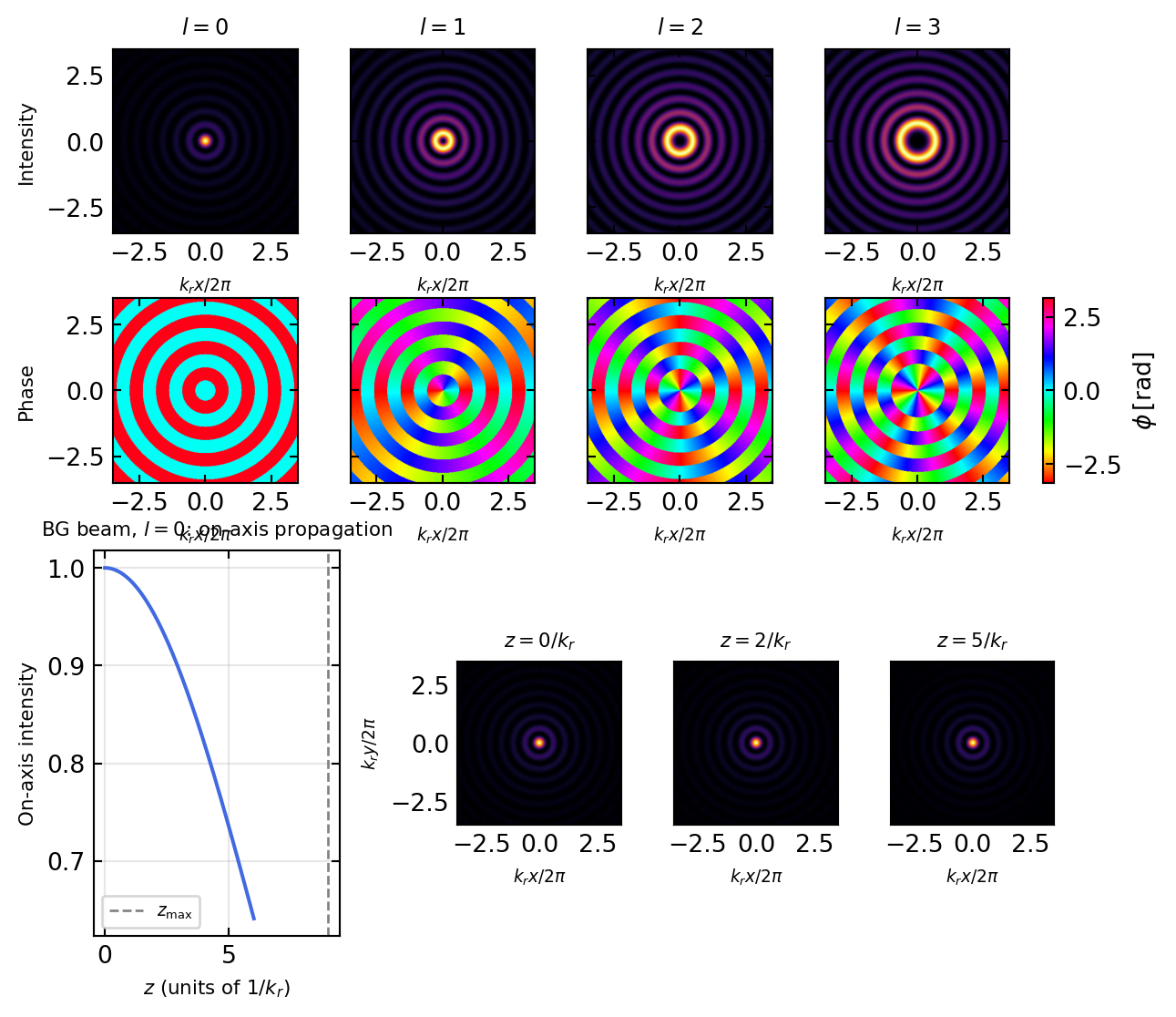
The top panels confirm that the \(l=0\) Bessel beam has a bright central spot surrounded by concentric rings of decreasing amplitude, while higher-order beams have a dark vortex core (intensity zero on axis for \(l \neq 0\)) and the characteristic \(l\)-fold phase winding visible in the phase maps. Note that the phase plot also displays radial \(\pi\)-jumps between successive intensity rings: because \(J_l(k_r r)\) is a real-valued oscillating function, it changes sign at each radial node, and that sign flip shows up in \(\arg(U_l)\) as a \(\pi\) shift. These jumps are physical, not a numerical artefact — they reflect the fact that an ideal Bessel beam is a coherent superposition of plane waves on a single cone, so its transverse amplitude is real and oscillatory rather than smoothly varying. The bottom panels show that the Bessel-Gaussian transverse profile is essentially preserved during propagation — only its overall brightness is modulated by the slowly varying envelope \(E(z)\) — maintaining its shape over the depth of field \(z_\text{max}\), after which the Gaussian damping causes the beam to fade.
Applications of Bessel and Bessel-Gaussian beams span a wide range of modern photonics: non-contact optical manipulation of particles over long distances, laser micro-machining of deep narrow channels (the elongated focal line drills material along \(z_\text{max}\)), light-sheet fluorescence microscopy (a Bessel illumination sheet provides higher axial resolution than a Gaussian sheet), and ultrafast laser filamentation in transparent media. Their orbital angular momentum variants (\(l \neq 0\)) are used in optical vortex trapping and quantum information encoding.
Applications of Gaussian and Higher-Order Beams
The structured beams discussed in this lecture are at the heart of a broad range of modern photonics applications.
Gaussian beams are the workhorse of laser optics. Their clean, analytically tractable profile makes them ideal for free-space communication links, laser ranging (LIDAR), and precision interferometry. In optical data storage (CD/DVD/Blu-ray) a tightly focused Gaussian spot writes and reads sub-micron features. In confocal and two-photon microscopy the diffraction-limited Gaussian focus confines excitation to a thin axial slice, providing intrinsic optical sectioning. Gaussian beams are also the natural output of single-mode optical fibers and diode-pumped solid-state lasers, so coupling efficiency between these systems is maximised when the beam parameters are matched.
Hermite-Gaussian (HG) beams arise naturally in laser cavities with rectangular (Fabry-Perot slab or rectangular mirror) symmetry. Mode-selective intracavity elements suppress higher-order HG modes to force single-mode (\(\text{TEM}_{00}\)) operation, while deliberate HG excitation finds use in laser material processing (shaping the ablation footprint) and in optical coherence tomography where higher-order modes improve depth sensitivity.
Laguerre-Gaussian (LG) beams carry orbital angular momentum (OAM) of \(l\hbar\) per photon, which can be transferred to microscopic objects. This makes them the tool of choice for optical spanners: a particle trapped off-axis orbits the beam axis at a rate set by \(l\) and the beam power. In quantum optics, the discrete OAM degree of freedom provides a high-dimensional Hilbert space for encoding quantum information, enabling entanglement in OAM modes. LG beams are also used in super-resolution STED microscopy, where the dark vortex core of an \(l=1\) beam serves as the depletion doughnut that suppresses fluorescence outside a sub-diffraction spot.
Bessel and Bessel-Gaussian beams exploit their non-diffracting character and self-healing property. An axicon-generated Bessel-Gaussian beam produces a long needle-like focus ideal for laser micro-drilling of high-aspect-ratio channels in glass. In light-sheet (selective-plane illumination) microscopy the Bessel illumination sheet maintains its thin waist over a far larger field of view than a Gaussian sheet, dramatically reducing out-of-focus photobleaching. The self-healing property allows the beam to reconstruct behind obscuring particles, which is exploited in optical manipulation of particles inside turbid media and in atmospheric propagation through partial obstructions.