The previous lecture established that any field at a plane \(z=0\) can be decomposed into plane waves via its Fourier transform, and that free-space propagation multiplies each component by the transfer function \(H(\nu_x,\nu_y;z) = e^{ik_z z}\). Here we apply this framework to the two central problems of optical imaging: how a lens performs an exact Fourier transform (enabling controlled spatial filtering), and how the finite aperture of any real system limits resolution through the point spread function and optical transfer function.
The Lens as a Fourier Transformer
The Fraunhofer result requires propagation distances \(z \gg \pi a^2/\lambda\) that are often impractically large. A thin lens solves this problem elegantly: it performs an exact Fourier transform at the finite distance of its focal length \(f\), with no approximation beyond the thin-lens and paraxial assumptions.
Derivation. Place an object with transmission \(t(x',y')\) in the front focal plane (at \(z=-f\), i.e. a distance \(f\) in front of the lens). For unit-amplitude plane-wave illumination the field just behind the object is \(U(x',y',{-f}) = t(x',y')\). Propagating this field by Fresnel from \(z=-f\) to the lens at \(z=0\), multiplying by the lens phase factor \(e^{-ik(x^2+y^2)/2f}\), and propagating a second Fresnel step from \(z=0\) to the back focal plane at \(z=+f\), the two quadratic phase factors — one from the Fresnel propagation and one from the lens — cancel exactly. The result is:
The back focal plane of a lens is the Fourier plane of its front focal plane. The spatial scale in the Fourier plane is \(\lambda f\): a high focal-length lens stretches the Fourier pattern across a larger area, while a short focal-length lens compresses it.
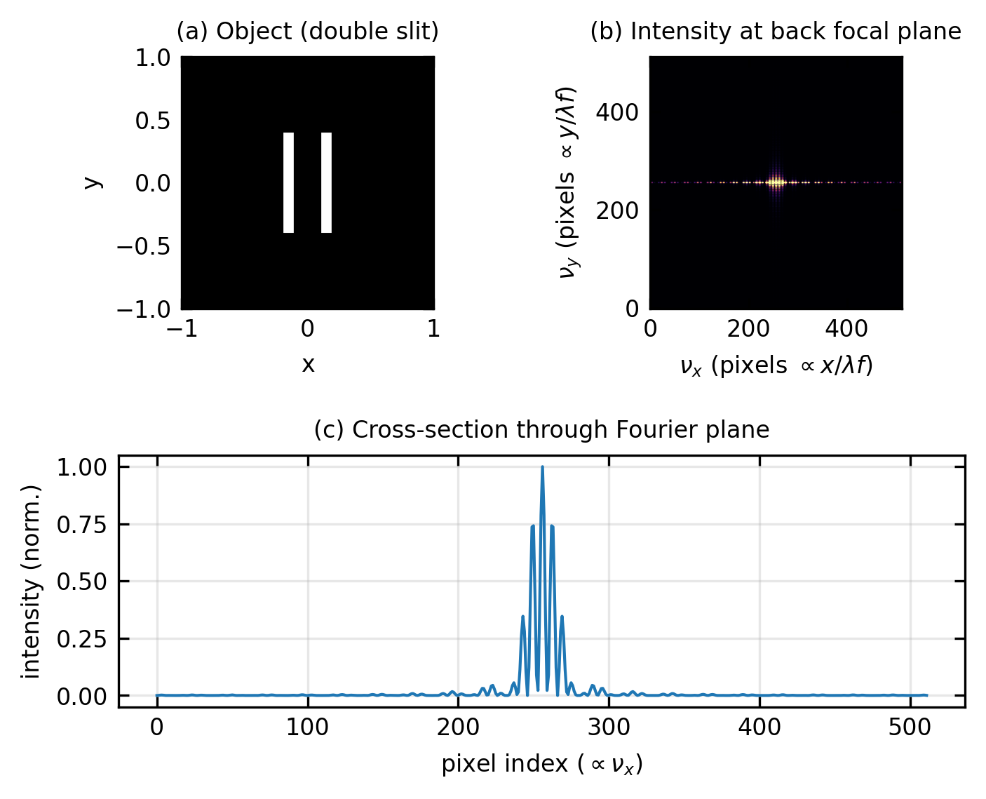
Figure 1— A thin lens performs a spatial Fourier transform. (a) Test object: a double slit. (b) Intensity at the back focal plane \(\propto|\hat{t}(\nu_x,\nu_y)|^2\), computed as the squared magnitude of the 2D FFT. The \(\cos^2\) interference fringes from the slit separation appear inside a sinc² envelope from the finite slit width. (c) Horizontal cross-section through the Fourier plane.
Spatial Filtering and the 4f System
The lens-FT result leads immediately to a practical optical processor: the 4f system. Two lenses, each of focal length \(f\), are placed coaxially with their focal planes coinciding at the midpoint. The object sits one focal length in front of lens 1; the image forms one focal length behind lens 2. The system spans a total length of \(4f\).
The shared focal plane between the two lenses is the Fourier plane. Because lens 1 performs the FT there, the field at the Fourier plane is \(\propto\hat{t}(\nu_x,\nu_y)\). Lens 2 then performs an inverse FT back to the image plane. In the absence of any modification:
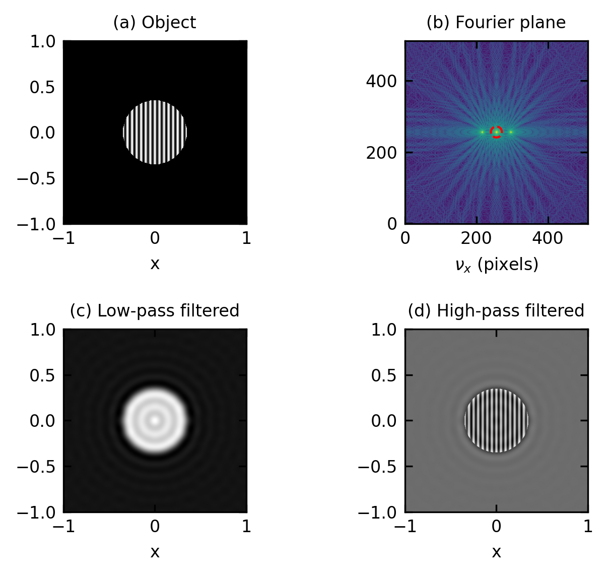
Figure 2— 4f spatial filtering demonstration. (a) Test object: a disk with a superimposed high-frequency grating. (b) Fourier plane spectrum; the dashed circle marks the low-pass cutoff \(\nu_c\). (c) Low-pass filtered image: the grating is removed, leaving a smooth disk. (d) High-pass filtered image: only the edges and fine texture survive.
The low-pass filter transmits only \(\nu_r < \nu_c\), smoothing the image by removing the high-frequency grating. The high-pass filter does the opposite: it blocks the DC and low-frequency components, leaving only sharp edges and fine texture. The disk boundary becomes a bright ring because it is where the high spatial frequencies are concentrated. This edge-enhancement is the basis of darkfield microscopy; the phase-contrast variant — shifting only the DC component by \(\pi/2\) — is the Zernike technique developed in the microscopy lectures.
Point Spread Function, Optical Transfer Function, and Resolution
The 4f filtering framework provides the natural language for characterising the imaging performance of any optical system.
Point Spread Function
The point spread function (PSF) \(h(x,y)\) is the image formed by the system of a single point source located at the origin of the object plane. In the Fourier framework it is the inverse Fourier transform of the system’s transfer function \(H(\nu_x,\nu_y)\):
\[h(x,y) = \mathcal{F}^{-1}\{H(\nu_x,\nu_y)\}\]
For a diffraction-limited system with a circular pupil of radius \(R\) (numerical aperture \(\mathrm{NA} = n\sin\theta_\mathrm{max}\)), the transfer function is a disk of radius \(\nu_\mathrm{max} = \mathrm{NA}/\lambda\) and the PSF is the Airy pattern:
\[h(r) \propto \left[\frac{2J_1(\pi D r/\lambda f)}{\pi D r/\lambda f}\right]^2\]
where \(D = 2R\) is the pupil diameter, \(f\) is the focal length, and \(r = \sqrt{x^2+y^2}\). The first zero of the Airy pattern falls at \(r_\mathrm{Airy} = 1.22\,\lambda f/D\), which is the Rayleigh resolution criterion: two point sources are just resolved when the peak of one coincides with the first zero of the other, giving a minimum resolvable distance
The Abbe diffraction limit arrives at the same scale from a different argument — the finest grating whose first diffraction order still enters the objective has period \(d_\mathrm{min} = \lambda/2\,\mathrm{NA}\) — giving
The two criteria agree to within a factor of \(\approx 1.2\) and both establish that no standard far-field optical system can resolve features finer than roughly \(\lambda / (2\,\mathrm{NA})\).
Image Formation as Convolution
Because the PSF is the impulse response of the imaging system, any linear, shift-invariant system maps an extended object \(f(x,y)\) to an image \(g(x,y)\) by convolution:
The function \(H(\nu_x,\nu_y)\) here is the optical transfer function (OTF). Its magnitude \(|H|\) is the modulation transfer function (MTF): it equals 1 at low frequencies, rolls off, and reaches zero at the diffraction cut-off \(\nu_\mathrm{max} = D/(\lambda f)\). The system therefore acts as a low-pass filter – spatial frequencies beyond \(\nu_\mathrm{max}\) are completely suppressed and the corresponding fine detail is lost from the image.
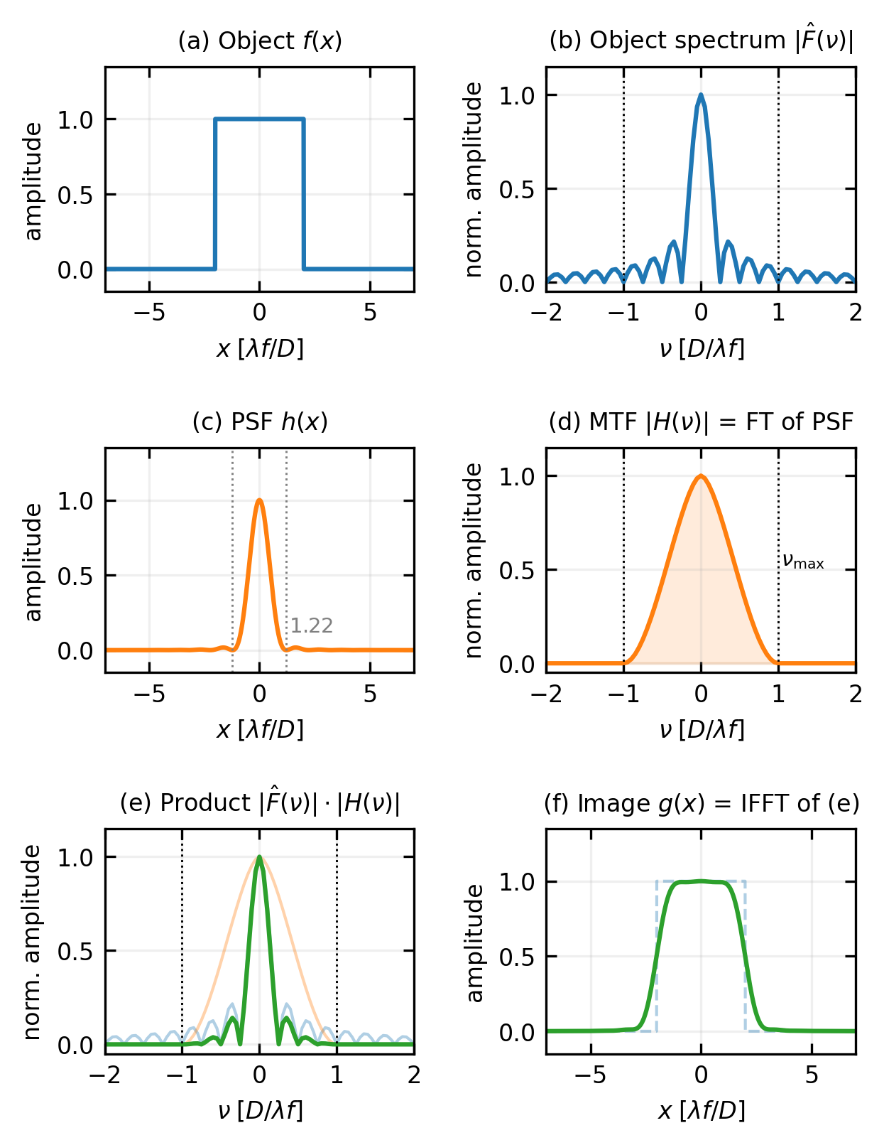
Figure 3 makes this concrete by tracing each step in both domains side by side. The left column shows the spatial domain directly: object \(f\), PSF \(h\), and image \(g = f * h\). The right column shows the same steps in the frequency domain: spectrum \(|\hat{F}|\), MTF \(|H|\), and their pointwise product \(|\hat{F}| \cdot |H|\). The inverse transform of that product recovers the image. The key is panel (f): the sinc-like object spectrum is truncated wherever the MTF reaches zero (dotted lines at \(\pm\nu_\mathrm{max}\)). The spatial consequence of this truncation is visible in panel (e) – the sharp edges of the rectangular object are rounded in the image because the high-frequency components that encode those edges have been removed.
Figure 3— Image formation as convolution, shown in two equivalent representations. Left column (spatial domain): (a) rectangular-bar object \(f(x)\), (c) PSF \(h(x)\) (1-D Airy profile, first zero at \(1.22\,\lambda f/D\)), (e) image \(g(x) = \mathcal{F}^{-1}\{\hat{F}\cdot H\}\) with the original object shown dashed for comparison – the sharp edges are rounded because their high-frequency content is removed. Right column (frequency domain): (b) object spectrum \(|\hat{F}(\nu)|\) (sinc-like, zeros every \(0.25\,D/\lambda f\)), (d) MTF \(|H(\nu)|\) with shaded passband ending at the diffraction cut-off \(\nu_\mathrm{max} = D/(\lambda f)\) (dotted), (f) the product \(|\hat{F}|\cdot|H|\) = image spectrum; components beyond \(\nu_\mathrm{max}\) are suppressed to zero.
Coherent vs. Incoherent Imaging
The convolution rule above comes in two distinct forms depending on whether the illumination is coherent (laser, single spatial mode) or incoherent (LED, thermal source, fluorescence).
Coherent imaging — the complex amplitude is the relevant quantity. The image amplitude is the convolution of the object amplitude with the coherent PSF:
The system’s transfer function acts directly on complex amplitudes, and the OTF is the pupil function itself (top-hat up to \(\nu_\mathrm{max}\), zero beyond). Phase of the object is preserved and contributes to image contrast.
Incoherent imaging — intensities add (no phase relationship between source points). The image intensity is the convolution of the object intensity with the incoherent PSF:
The incoherent OTF is the autocorrelation of the pupil function, which extends to twice the coherent cut-off (\(2\nu_\mathrm{max}\)) but with reduced contrast at high frequencies. Despite the wider bandwidth, incoherent systems do not always produce sharper images than coherent systems — the MTF rolloff and the absence of phase contrast mean the two regimes are suited to different tasks.
Property
Coherent
Incoherent
Superposition
Amplitudes
Intensities
PSF
\(h(x,y)\) (complex)
\(|h(x,y)|^2\) (real, positive)
OTF
Pupil function
Autocorrelation of pupil
Bandwidth
\(\nu_\mathrm{max}\)
\(2\nu_\mathrm{max}\)
Phase sensitivity
Yes
No
Typical source
Laser, SLM
LED, fluorescence, white light
Fluorescence microscopy is inherently incoherent (each fluorophore emits independently), which is one reason it achieves clean, artefact-free images. Coherent systems such as holographic or interferometric microscopes recover phase and thus reveal refractive-index variations invisible to incoherent methods. The superresolution techniques discussed in later lectures (STED, STORM, SIM) each exploit specific aspects of this coherent/incoherent distinction.