Electro-Optics & Acousto-Optics

Introduction: Controlling Light with External Fields

In the previous lecture we saw that anisotropic materials — crystals with direction-dependent refractive indices — split light into ordinary and extraordinary rays and enable devices like wave plates. A natural next question is: can we control this anisotropy dynamically?

The answer is yes, and it leads to two of the most important families of active optical devices:

• Electro-optic (EO) devices use an applied electric field to modify the refractive index tensor of a crystal. This allows fast (GHz) switching of polarization, phase, and amplitude.
• Acousto-optic (AO) devices use a sound wave to create a periodic refractive index grating inside a medium. Light diffracts off this grating, enabling frequency shifting, beam deflection, and intensity modulation.

Both can be understood as perturbations of the dielectric tensor: the EO effect modifies it uniformly, the AO effect modifies it periodically. Both are essential building blocks in modern photonics: laser Q-switching, optical telecommunications, microscopy (AO beam scanning, SLMs for wavefront shaping), and spectroscopy.

These devices also connect directly to the physics of the Nonlinear Optics lecture. There we expanded the polarization of a medium as a power series in the driving field, \(P = \varepsilon_0\left(\chi^{(1)}E + \chi^{(2)}E^2 + \chi^{(3)}E^3 + \cdots\right)\), and saw how the higher-order terms let one wave mix with another. Electro-optics is the same expansion read with a different field: instead of a second strong optical wave, we apply a quasi-static voltage, so that the refractive index seen by the light becomes something we control electronically. The Pockels effect turns out to be exactly the \(\chi^{(2)}\) term of that expansion and the electro-optic Kerr effect a \(\chi^{(3)}\) term, which is why the same symmetry rules and the same crystals reappear here.

---

Part I: Electro-Optics

1. The Electro-Optic Effect

Physical Origin

When an external electric field \(\mathbf{E}_\text{ext}\) is applied to a crystal, it displaces the ionic sublattices and distorts the electron clouds, changing the polarizability and hence the refractive index. The effect can be expanded in powers of the applied field:

\[ \Delta\left(\frac{1}{n^2}\right)_{ij} = r_{ijk}\, E_k + s_{ijkl}\, E_k E_l + \cdots \tag{1.1}\]

where:

• \(r_{ijk}\) is the linear electro-optic (Pockels) tensor — a third-rank tensor
• \(s_{ijkl}\) is the quadratic electro-optic (Kerr) tensor — a fourth-rank tensor

The Pockels effect (\(\propto E\)) exists only in non-centrosymmetric crystals (no inversion symmetry), while the Kerr effect (\(\propto E^2\)) exists in all materials, including liquids and glasses.

This expansion is the static-field face of the nonlinear polarization series \(P = \varepsilon_0\left(\chi^{(1)}E + \chi^{(2)}E^2 + \chi^{(3)}E^3 + \cdots\right)\) introduced in the Nonlinear Optics lecture. When one of the two fields driving a \(\chi^{(2)}\) process is a static field \(E(0)\) instead of a second optical wave, the second-order polarization \(P(\omega) \propto \chi^{(2)} E(0)\, E(\omega)\) rescales the index seen at the optical frequency by an amount linear in \(E(0)\). That linear-in-voltage index change is the Pockels effect, so the Pockels tensor \(r\) is set by the same \(\chi^{(2)}\) that drives second-harmonic generation. Because \(\chi^{(2)}\) vanishes in any medium with a center of inversion, so does the Pockels effect, which is the same selection rule that forbids second-harmonic generation in centrosymmetric materials. The quadratic term needs two applied fields and is a \(\chi^{(3)}\) process, so it carries no symmetry restriction and survives in glasses and liquids.

The Index Ellipsoid

The refractive index properties of an anisotropic crystal are described by the index ellipsoid (or indicatrix):

\[ \frac{x^2}{n_x^2} + \frac{y^2}{n_y^2} + \frac{z^2}{n_z^2} = 1 \tag{1.2}\]

An applied electric field deforms this ellipsoid. For the Pockels effect in contracted notation, the change is:

\[ \Delta\left(\frac{1}{n^2}\right)_i = \sum_{j=1}^{3} r_{ij}\, E_j \tag{1.3}\]

where \(i = 1, \ldots, 6\) runs over the independent components of the symmetric impermeability tensor (using Voigt notation) and \(r_{ij}\) is the \(6 \times 3\) electro-optic tensor.

2. The Pockels Effect

Key Materials

Table 1.1— Common electro-optic crystals and their Pockels coefficients.

Crystal	Symmetry	Key coefficient	\(n_o\)	\(n_e\)
LiNbO\(_3\)	Trigonal 3m	\(r_{33} = 30.8\) pm/V	2.286	2.200
KDP (KH\(_2\)PO\(_4\))	Tetragonal \(\bar{4}2m\)	\(r_{63} = 10.6\) pm/V	1.514	1.472
BBO (\(\beta\)-BaB\(_2\)O\(_4\))	Trigonal 3m	\(r_{22} = 2.7\) pm/V	1.677	1.553
GaAs	Cubic \(\bar{4}3m\)	\(r_{41} = 1.6\) pm/V	3.37	—

It is no coincidence that LiNbO\(_3\), KDP and BBO appear in this table: they are the same crystals used for phase-matched second-harmonic generation in the Nonlinear Optics lecture. The strong, non-vanishing \(\chi^{(2)}\) that makes them efficient frequency converters is exactly what gives them a large Pockels response.

Phase Modulation

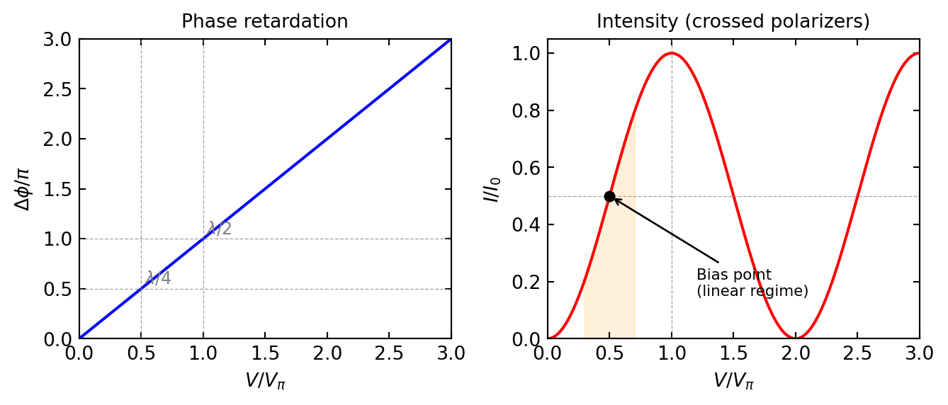
The most common configuration uses a longitudinal field (field parallel to light propagation along the optic axis \(z\)). For a crystal of length \(L\) with applied voltage \(V = E_z \cdot L\), the induced phase difference between the two polarization eigenmodes is:

\[ \Delta\phi = \frac{2\pi}{\lambda}\, n_o^3\, r_{63}\, \frac{V}{d}\, L = \pi \frac{V}{V_\pi} \tag{1.4}\]

where the half-wave voltage \(V_\pi\) is the voltage needed to produce a \(\pi\) phase shift:

\[ V_\pi = \frac{\lambda\, d}{2\, n_o^3\, r_{63}\, L} \tag{1.5}\]

For a transverse configuration (\(E \perp k\)), \(V_\pi\) can be reduced by increasing the aspect ratio \(L/d\).

fig, axes = plt.subplots(1, 2, figsize=get_size(18, 8))

V_Vpi = np.linspace(0, 3, 500)

# Left: Phase retardation
ax = axes[0]
delta_phi = np.pi * V_Vpi
ax.plot(V_Vpi, delta_phi / np.pi, 'b-', linewidth=1.5)
ax.axhline(y=0.5, color='gray', linestyle='--', linewidth=0.5, alpha=0.7)
ax.axhline(y=1.0, color='gray', linestyle='--', linewidth=0.5, alpha=0.7)
ax.axvline(x=0.5, color='gray', linestyle='--', linewidth=0.5, alpha=0.7)
ax.axvline(x=1.0, color='gray', linestyle='--', linewidth=0.5, alpha=0.7)
ax.set_xlabel(r'$V / V_\pi$')
ax.set_ylabel(r'$\Delta\phi / \pi$')
ax.set_title('Phase retardation', fontsize=10)
ax.set_xlim(0, 3)
ax.set_ylim(0, 3)
ax.text(0.52, 0.55, r'$\lambda/4$', fontsize=9, color='gray')
ax.text(1.02, 1.05, r'$\lambda/2$', fontsize=9, color='gray')

# Right: Intensity modulation (crossed polarizers)
ax = axes[1]
I_transmitted = np.sin(np.pi * V_Vpi / 2)**2
ax.plot(V_Vpi, I_transmitted, 'r-', linewidth=1.5)
ax.axhline(y=0.5, color='gray', linestyle='--', linewidth=0.5, alpha=0.7)
ax.axvline(x=1.0, color='gray', linestyle='--', linewidth=0.5, alpha=0.7)

# Mark operating point
V_bias = 0.5
I_bias = np.sin(np.pi * V_bias / 2)**2
ax.plot(V_bias, I_bias, 'ko', markersize=5)
ax.annotate('Bias point\n(linear regime)',
            xy=(V_bias, I_bias), xytext=(1.2, 0.15),
            arrowprops=dict(arrowstyle='->', color='black'),
            fontsize=8)

# Show linear modulation region
V_mod = np.linspace(0.3, 0.7, 100)
I_mod = np.sin(np.pi * V_mod / 2)**2
ax.fill_between(V_mod, 0, I_mod, alpha=0.15, color='orange')

ax.set_xlabel(r'$V / V_\pi$')
ax.set_ylabel(r'$I / I_0$')
ax.set_title('Intensity (crossed polarizers)', fontsize=10)
ax.set_xlim(0, 3)
ax.set_ylim(0, 1.05)

plt.tight_layout()
plt.show()

Figure 1.1— Pockels effect: phase retardation and transmitted intensity as a function of applied voltage. Left: the induced birefringence creates a voltage-dependent phase shift between polarization components. Right: between crossed polarizers, the transmitted intensity follows \(I/I_0 = \sin^2(\pi V / 2V_\pi)\), enabling amplitude modulation.

3. The Kerr Effect

The quadratic (Kerr) electro-optic effect exists in all materials, including isotropic ones like glass and liquids. The induced birefringence is:

\[ \Delta n = \lambda\, K\, E^2 \tag{1.6}\]

where \(K\) is the Kerr constant (units: m/V\(^2\)). Typical values: \(K \approx 3.6 \times 10^{-12}\) m/V\(^2\) for nitrobenzene, \(K \approx 4.4 \times 10^{-14}\) m/V\(^2\) for water.

The Kerr effect is important in:

• Kerr cells for ultrafast shutters (sub-picosecond response in liquids)
• Self-phase modulation in optical fibers, where the light’s own field plays the role of \(E\) (the optical Kerr effect)
• Kerr lens mode-locking in ultrafast lasers

The last two of these point straight back to nonlinear optics. The electro-optic Kerr effect of Equation 1.6 and the optical Kerr effect are both governed by the third-order susceptibility \(\chi^{(3)}\); they differ only in what supplies the field. Here a slowly varying applied voltage produces the static birefringence \(\Delta n \propto E^2\), whereas in self-phase modulation the intense light field itself plays the role of \(E\) and modulates its own index as \(\Delta n = n_2 I\). Seeing them as one effect is useful, because the Kerr constant \(K\) measured with a voltage and the nonlinear index \(n_2\) measured with an intense beam probe the same underlying nonlinearity.

fig, axes = plt.subplots(1, 2, figsize=get_size(18, 8))

E = np.linspace(-1, 1, 500)  # Normalized field (E/E_pi)

# Left: Birefringence
ax = axes[0]
dn_pockels = E          # Linear
dn_kerr = E**2           # Quadratic
ax.plot(E, dn_pockels, 'b-', linewidth=1.5, label='Pockels ($\\propto E$)')
ax.plot(E, dn_kerr, 'r-', linewidth=1.5, label='Kerr ($\\propto E^2$)')
ax.axhline(y=0, color='k', linewidth=0.3)
ax.axvline(x=0, color='k', linewidth=0.3)
ax.set_xlabel(r'Applied field $E$ (norm.)')
ax.set_ylabel(r'$\Delta n$ (norm.)')
ax.set_title('Induced birefringence', fontsize=10)
ax.legend(fontsize=8, frameon=False)

# Right: Transmission
ax = axes[1]
# Pockels: T = sin²(π/2 * E/E_pi) — using E_pi = 1
T_pockels = np.sin(np.pi / 2 * np.abs(E))**2
# Kerr: T = sin²(π/2 * (E/E_pi)²)
T_kerr = np.sin(np.pi / 2 * E**2)**2
ax.plot(E, T_pockels, 'b-', linewidth=1.5, label='Pockels')
ax.plot(E, T_kerr, 'r-', linewidth=1.5, label='Kerr')
ax.set_xlabel(r'Applied field $E$ (norm.)')
ax.set_ylabel(r'$T$ (crossed polarizers)')
ax.set_title('Transmission', fontsize=10)
ax.legend(fontsize=8, frameon=False)

plt.tight_layout()
plt.show()

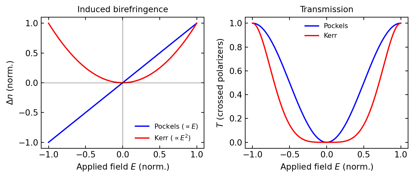
Figure 1.2— Comparison of Pockels (linear) and Kerr (quadratic) electro-optic effects. Left: induced birefringence \(\Delta n\) as a function of applied field. The Pockels effect is linear and changes sign with the field; the Kerr effect is quadratic and always positive. Right: corresponding transmission through crossed polarizers.

4. EO Applications

Pockels Cell — Polarization and Amplitude Modulation

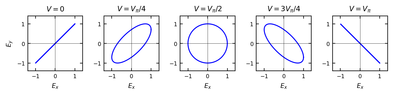
A Pockels cell consists of an EO crystal placed between two polarizers. By varying the applied voltage, the polarization state exiting the crystal changes continuously from linear → elliptical → circular → elliptical → linear (rotated 90°). Between crossed polarizers, this converts to amplitude modulation.

Applications:

• Q-switching of pulsed lasers (nanosecond switching)
• Cavity dumping for ultrashort pulse extraction
• Optical telecommunications (GHz intensity modulation in LiNbO\(_3\) Mach-Zehnder modulators)
• Spatial light modulators (SLMs) using liquid crystal arrays — each pixel is an independently addressable EO cell

Mach-Zehnder Modulator

Modern optical communications use integrated LiNbO\(_3\) Mach-Zehnder interferometers where the EO effect shifts the phase in one arm. The output intensity is:

\[ I = I_0 \cos^2\!\left(\frac{\pi V}{2 V_\pi}\right) \]

This provides linear modulation around the quadrature bias point \(V = V_\pi/2\).

fig, axes = plt.subplots(1, 5, figsize=get_size(18, 5))

voltages = [0, 0.25, 0.5, 0.75, 1.0]
labels = [r'$0$', r'$V_\pi/4$', r'$V_\pi/2$', r'$3V_\pi/4$', r'$V_\pi$']

t = np.linspace(0, 2 * np.pi, 200)

for ax, V_frac, label in zip(axes, voltages, labels):
    delta = np.pi * V_frac  # Phase retardation
    Ex = np.cos(t)
    Ey = np.cos(t + delta)

    ax.plot(Ex, Ey, 'b-', linewidth=1.2)
    ax.set_xlim(-1.4, 1.4)
    ax.set_ylim(-1.4, 1.4)
    ax.set_aspect('equal')
    ax.axhline(0, color='k', linewidth=0.3)
    ax.axvline(0, color='k', linewidth=0.3)
    ax.set_title(f'$V = {label[1:-1]}$', fontsize=9)
    ax.set_xlabel(r'$E_x$', fontsize=8)
    if V_frac == 0:
        ax.set_ylabel(r'$E_y$', fontsize=8)
    ax.tick_params(labelsize=7)

plt.tight_layout()
plt.show()

Figure 1.3— Polarization state evolution through a Pockels cell as voltage increases from \(0\) to \(V_\pi\). At \(V = 0\) the light is linearly polarized (input). At \(V_\pi/4\) it becomes elliptical, at \(V_\pi/2\) circular, and at \(V_\pi\) it is linear again but rotated by 90° — fully transmitted by a crossed analyzer.

---

Part II: Acousto-Optics

5. Sound Waves as Refractive Index Gratings

An acoustic wave propagating through a transparent medium creates a periodic modulation of the density, and hence of the refractive index:

\[ n(x, t) = n_0 + \Delta n \sin(\Omega t - K x) \tag{2.1}\]

where \(\Omega = 2\pi f_s\) is the sound angular frequency, \(K = 2\pi / \Lambda\) is the acoustic wavevector, \(\Lambda\) is the acoustic wavelength, and \(\Delta n\) is the amplitude of the index modulation (typically \(\Delta n \sim 10^{-5}\) to \(10^{-4}\)).

This periodic structure acts as a phase diffraction grating for light. Because the grating is moving (at the speed of sound \(v_s = \Lambda f_s\)), it also shifts the frequency of the diffracted light — a key difference from static gratings.

The Photoelastic Effect

The index modulation arises from the photoelastic (elasto-optic) effect:

\[ \Delta n = -\frac{1}{2}\, n_0^3\, p\, S \tag{2.2}\]

where \(p\) is the relevant photoelastic coefficient and \(S\) is the acoustic strain amplitude.

6. Bragg Diffraction

When the acoustic wavelength \(\Lambda\) is much larger than the optical wavelength \(\lambda\) and the interaction length \(L\) is long enough, we enter the Bragg regime. The condition for strong diffraction is given by the Klein-Cook parameter:

\[ Q = \frac{2\pi \lambda L}{n_0 \Lambda^2} \gg 1 \tag{2.3}\]

In this regime, efficient diffraction occurs only at the Bragg angle:

\[ \sin\theta_B = \frac{\lambda}{2 n_0 \Lambda} = \frac{K}{2k} \tag{2.4}\]

This is exactly the condition for momentum conservation (phase matching) between the incident photon, the diffracted photon, and the acoustic phonon:

\[ \mathbf{k}_\text{diffracted} = \mathbf{k}_\text{incident} \pm \mathbf{K} \tag{2.5}\]

The \(\pm\) corresponds to diffraction into the +1 or −1 order, and energy conservation requires:

\[ \omega_\text{diffracted} = \omega_\text{incident} \pm \Omega \tag{2.6}\]

The diffracted beam is frequency-shifted by \(\pm f_s\) (typically 40–400 MHz).

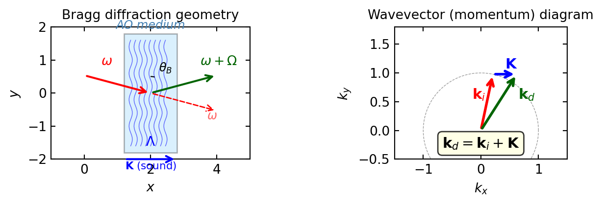
This pair of conditions, momentum conservation \(\mathbf{k}_d = \mathbf{k}_i \pm \mathbf{K}\) together with energy conservation \(\omega_d = \omega \pm \Omega\), is the same three-wave phase matching that governs the \(\chi^{(2)}\) processes of the Nonlinear Optics lecture. The only difference is that the third wave is an acoustic phonon rather than an optical photon, so the diffracted light is shifted by the small sound frequency instead of being combined into a new optical wave. In this sense an acousto-optic frequency shifter is the phononic counterpart of sum- and difference-frequency generation: up-shifting absorbs a phonon, down-shifting emits one.

fig, axes = plt.subplots(1, 2, figsize=get_size(18, 6))

# --- Left panel: Physical geometry ---
ax = axes[0]
ax.set_xlim(-1, 5)
ax.set_ylim(-2, 2)
ax.set_aspect('equal')

# Draw the AO medium
rect = Rectangle((1.2, -1.8), 1.6, 3.6, facecolor='lightskyblue', edgecolor='black',
                  alpha=0.3, linewidth=1)
ax.add_patch(rect)

# Draw acoustic wavefronts (vertical lines inside medium)
n_fronts = 8
for i in range(n_fronts):
    x_pos = 1.4 + i * (1.2 / n_fronts)
    # Slight sinusoidal distortion to show it's a wave
    y_line = np.linspace(-1.6, 1.6, 50)
    x_line = x_pos + 0.05 * np.sin(2 * np.pi * y_line / 0.8)
    ax.plot(x_line, y_line, 'b-', linewidth=0.5, alpha=0.6)

# Sound wave arrow
ax.annotate('', xy=(2.8, -2.0), xytext=(1.2, -2.0),
            arrowprops=dict(arrowstyle='->', color='blue', lw=1.5))
ax.text(2.0, -2.3, r'$\mathbf{K}$ (sound)', fontsize=8, ha='center', color='blue')

# Incident beam
theta_B = 15 * np.pi / 180
x_in = np.array([0, 2.0])
y_in = np.array([np.tan(theta_B) * 2.0, 0])
ax.annotate('', xy=(2.0, 0), xytext=(0, np.tan(theta_B) * 2.0),
            arrowprops=dict(arrowstyle='->', color='red', lw=1.5))
ax.text(0.5, 0.85, r'$\omega$', fontsize=10, color='red')

# Diffracted beam (upshifted)
ax.annotate('', xy=(4.0, np.tan(theta_B) * 2.0), xytext=(2.0, 0),
            arrowprops=dict(arrowstyle='->', color='darkgreen', lw=1.5))
ax.text(3.5, 0.85, r'$\omega + \Omega$', fontsize=10, color='darkgreen')

# Transmitted beam (undiffracted, straight through)
ax.annotate('', xy=(4.0, -np.tan(theta_B) * 2.0), xytext=(2.0, 0),
            arrowprops=dict(arrowstyle='->', color='red', lw=1, linestyle='--'))
ax.text(3.7, -0.8, r'$\omega$', fontsize=9, color='red', alpha=0.6)

# Bragg angle annotation
from matplotlib.patches import Arc
arc = Arc((2.0, 0), 1.0, 1.0, angle=0, theta1=90 - 15, theta2=90, color='black', lw=0.8)
ax.add_patch(arc)
ax.text(2.25, 0.65, r'$\theta_B$', fontsize=9)

# Labels
ax.text(2.0, 1.95, 'AO medium', fontsize=9, ha='center',
        style='italic', color='steelblue')
ax.text(2.0, -1.6, r'$\Lambda$', fontsize=10, ha='center', color='blue')
ax.set_xlabel(r'$x$')
ax.set_ylabel(r'$y$')
ax.set_title('Bragg diffraction geometry', fontsize=10)

# --- Right panel: Wavevector diagram ---
ax2 = axes[1]
ax2.set_xlim(-1.5, 1.5)
ax2.set_ylim(-0.5, 1.8)
ax2.set_aspect('equal')

# Parameters
k = 1.0  # Optical wavevector magnitude
theta_B_rad = 12 * np.pi / 180

# Incident wavevector
kix = k * np.sin(theta_B_rad)
kiy = k * np.cos(theta_B_rad)
ax2.annotate('', xy=(kix, kiy), xytext=(0, 0),
            arrowprops=dict(arrowstyle='->', color='red', lw=2))
ax2.text(-0.15, 0.55, r'$\mathbf{k}_i$', fontsize=11, color='red')

# Acoustic wavevector (horizontal)
K_mag = 2 * k * np.sin(theta_B_rad)
ax2.annotate('', xy=(kix + K_mag, kiy), xytext=(kix, kiy),
            arrowprops=dict(arrowstyle='->', color='blue', lw=2))
ax2.text(kix + K_mag / 2, kiy + 0.1, r'$\mathbf{K}$', fontsize=11, color='blue')

# Diffracted wavevector
kdx = kix + K_mag
kdy = kiy
ax2.annotate('', xy=(kdx, kdy), xytext=(0, 0),
            arrowprops=dict(arrowstyle='->', color='darkgreen', lw=2))
ax2.text(0.65, 0.55, r'$\mathbf{k}_d$', fontsize=11, color='darkgreen')

# Show equal magnitudes with dashed circle
theta_circle = np.linspace(0, 2 * np.pi, 200)
ax2.plot(k * np.cos(theta_circle), k * np.sin(theta_circle),
         'k--', linewidth=0.5, alpha=0.4)

# Phase matching equation
ax2.text(0.0, -0.3, r'$\mathbf{k}_d = \mathbf{k}_i + \mathbf{K}$',
         fontsize=11, ha='center',
         bbox=dict(boxstyle='round,pad=0.3', facecolor='lightyellow', alpha=0.8))

ax2.set_xlabel(r'$k_x$')
ax2.set_ylabel(r'$k_y$')
ax2.set_title('Wavevector (momentum) diagram', fontsize=10)

plt.tight_layout()
plt.show()

Figure 2.1— Acousto-optic Bragg diffraction. Left: geometry showing incident beam at Bragg angle \(\\theta_B\) diffracted by a sound wave grating of wavelength \(\\Lambda\). The diffracted beam is frequency-shifted by \(\\pm f_s\). Right: momentum (wavevector) diagram — the acoustic wavevector \(\\mathbf{K}\) connects the incident and diffracted optical wavevectors, satisfying phase matching.

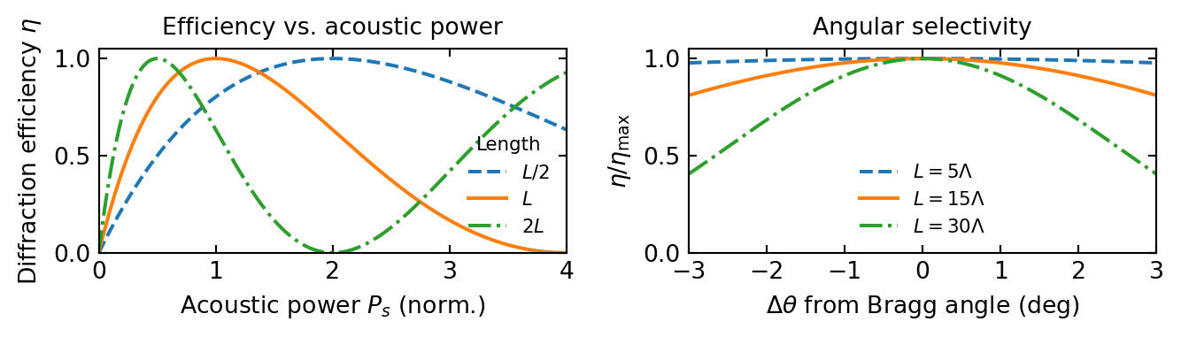
7. Diffraction Efficiency

In the Bragg regime, the diffraction efficiency (fraction of incident power diffracted into the first order) is:

\[ \eta = \sin^2\!\left(\frac{\pi \Delta n\, L}{\lambda \cos\theta_B}\right) = \sin^2\!\left(\frac{\pi}{\lambda \cos\theta_B}\sqrt{\frac{M_2\, P_s\, L}{2 H}}\right) \tag{2.7}\]

where \(P_s\) is the acoustic power, \(H\) is the transducer height, and \(M_2 = n_0^6 p^2 / (\rho v_s^3)\) is the acousto-optic figure of merit — a material property that determines how efficiently sound modulates light.

Table 2.1— Acousto-optic figures of merit for common materials.

Material	\(M_2\) (\(10^{-15}\) s\(^3\)/kg)	\(v_s\) (m/s)	Application
TeO\(_2\)	34.5	617	Deflectors, tunable filters
PbMoO\(_4\)	36.3	3630	Modulators
Fused silica	1.51	5960	UV applications
Ge	180	5500	IR modulators
Water	126	1500	Microscopy

fig, axes = plt.subplots(1, 2, figsize=get_size(18, 5.5))

# Left: Efficiency vs acoustic power
ax = axes[0]
P_norm = np.linspace(0, 4, 500)  # Normalized acoustic power

for L_factor, ls, label in [(0.5, '--', r'$L/2$'), (1.0, '-', r'$L$'), (2.0, '-.', r'$2L$')]:
    eta = np.sin(np.pi / 2 * np.sqrt(P_norm * L_factor))**2
    ax.plot(P_norm, eta, ls, linewidth=1.5, label=label)

ax.set_xlabel(r'Acoustic power $P_s$ (norm.)')
ax.set_ylabel(r'Diffraction efficiency $\eta$')
ax.set_title('Efficiency vs. acoustic power', fontsize=10)
ax.legend(fontsize=8, frameon=False, title='Length', title_fontsize=8)
ax.set_xlim(0, 4)
ax.set_ylim(0, 1.05)

# Right: Angular selectivity
ax = axes[1]
delta_theta = np.linspace(-3, 3, 500)  # In units of Lambda/L

for L_factor, ls, label in [(5, '--', '$L = 5\\Lambda$'),
                              (15, '-', '$L = 15\\Lambda$'),
                              (30, '-.', '$L = 30\\Lambda$')]:
    # sinc² angular dependence
    arg = L_factor * delta_theta * np.pi / 180
    eta_angular = np.sinc(arg / np.pi)**2
    ax.plot(delta_theta, eta_angular, ls, linewidth=1.5, label=label)

ax.set_xlabel(r'$\Delta\theta$ from Bragg angle (deg)')
ax.set_ylabel(r'$\eta / \eta_\mathrm{max}$')
ax.set_title('Angular selectivity', fontsize=10)
ax.legend(fontsize=8, frameon=False)
ax.set_xlim(-3, 3)
ax.set_ylim(0, 1.05)

plt.tight_layout()
plt.show()

Figure 2.2— Acousto-optic diffraction efficiency. Left: efficiency \(\\eta\) as a function of acoustic power for different interaction lengths, showing the \(\\sin^2\) dependence. 100% diffraction is achievable. Right: angular selectivity — the diffraction efficiency drops sharply when the incidence angle deviates from the Bragg angle, with selectivity improving for longer interaction lengths.

8. AO Devices and Applications

AO Modulator (AOM)

Switches beam on/off by deflecting it into the first diffraction order. Switching time \(\tau \approx d / v_s\) where \(d\) is the beam diameter — typically 10–100 ns.

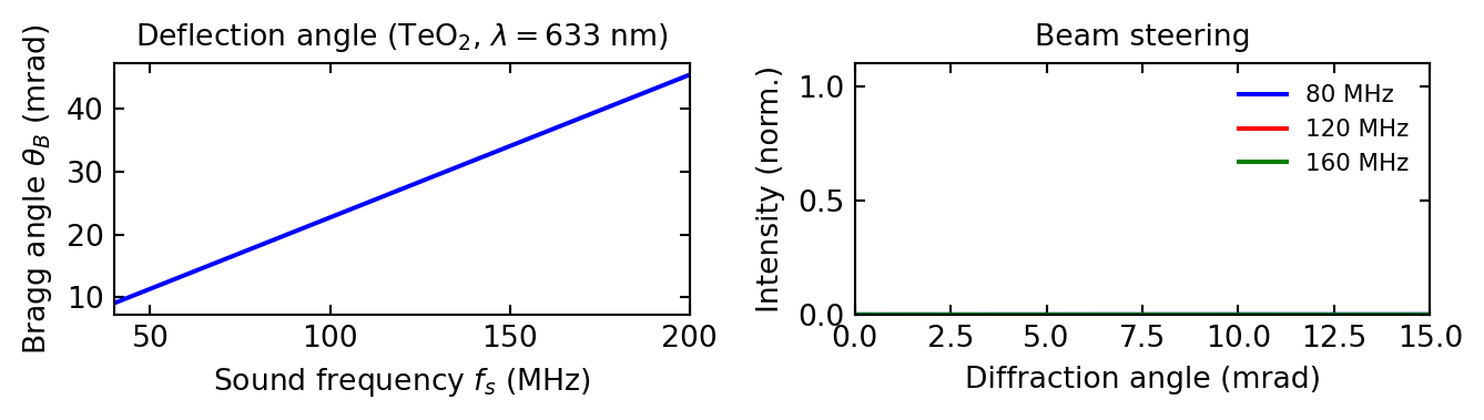
AO Deflector (AOD)

By varying the sound frequency \(f_s\), the Bragg angle changes, scanning the diffracted beam over an angular range \(\Delta\theta \propto \Delta f_s\). The number of resolvable spots is \(N = \tau \cdot \Delta f_s\) (time-bandwidth product).

AO Tunable Filter (AOTF)

Selects a narrow spectral band from broadband light — only the wavelength satisfying the Bragg condition at the given sound frequency is diffracted.

AO Frequency Shifter

The diffracted beam is shifted by exactly \(\pm f_s\). Used in heterodyne detection, laser Doppler velocimetry, and optical frequency comb stabilization.

fig, axes = plt.subplots(1, 2, figsize=get_size(18, 5.5))

# Parameters for TeO2
n0 = 2.26
vs = 617       # m/s in TeO2
lam = 633e-9   # wavelength in m

# Left: Deflection angle vs frequency
ax = axes[0]
f_s = np.linspace(40e6, 200e6, 500)  # 40-200 MHz
Lambda = vs / f_s
theta_B = np.arcsin(lam / (2 * n0 * Lambda))
theta_B_mrad = theta_B * 1e3

ax.plot(f_s / 1e6, theta_B_mrad, 'b-', linewidth=1.5)
ax.set_xlabel('Sound frequency $f_s$ (MHz)')
ax.set_ylabel(r'Bragg angle $\theta_B$ (mrad)')
ax.set_title(r'Deflection angle (TeO$_2$, $\lambda = 633$ nm)', fontsize=10)
ax.set_xlim(40, 200)

# Right: Beam profiles at different frequencies
ax = axes[1]
theta_range = np.linspace(0, 15, 1000)  # mrad

for freq, color, label in [(80e6, 'blue', '80 MHz'),
                             (120e6, 'red', '120 MHz'),
                             (160e6, 'green', '160 MHz')]:
    Lambda_f = vs / freq
    theta_center = np.arcsin(lam / (2 * n0 * Lambda_f)) * 1e3  # mrad
    # Gaussian beam profile
    beam_width = 0.8  # mrad
    profile = np.exp(-(theta_range - theta_center)**2 / (2 * beam_width**2))
    ax.plot(theta_range, profile, color=color, linewidth=1.5, label=label)
    ax.axvline(theta_center, color=color, linewidth=0.5, linestyle='--', alpha=0.5)

ax.set_xlabel(r'Diffraction angle (mrad)')
ax.set_ylabel('Intensity (norm.)')
ax.set_title('Beam steering', fontsize=10)
ax.legend(fontsize=8, frameon=False)
ax.set_xlim(0, 15)
ax.set_ylim(0, 1.1)

plt.tight_layout()
plt.show()

Figure 2.3— Acousto-optic deflector: changing the sound frequency \(f_s\) changes the Bragg angle and steers the diffracted beam. Left: deflection angle as a function of sound frequency for TeO\(_2\) at \(\\lambda = 633\) nm. Right: diffracted beam intensity profiles at three different RF frequencies, showing beam steering.

---

9. Connection to Fourier Optics

Both electro-optic and acousto-optic effects have a deep connection to the Fourier optics framework that we will develop in the next lecture:

Acousto-optic diffraction is spatial frequency manipulation. The sound wave creates a sinusoidal phase grating with spatial frequency \(K = 2\pi/\Lambda\). When light passes through, new spatial frequency components appear in the transmitted field at \(k_x \pm K\). This is a direct Fourier shift — the acoustic grating translates the optical spectrum in \(k\)-space.

Electro-optic phase modulation is temporal frequency manipulation. A sinusoidally driven Pockels cell modulates the phase at frequency \(\Omega\), creating new spectral sidebands at \(\omega \pm \Omega\). In the time-frequency Fourier domain, this is again a shift theorem.

Both devices therefore act as frequency mixers — one in the spatial domain, the other in the temporal domain. This perspective will be central when we discuss structured illumination microscopy (SIM), where a spatial frequency grating extends the observable passband of the microscope.

Summary Table

Property	Electro-Optic (Pockels)	Electro-Optic (Kerr)	Acousto-Optic
Effect	\(\Delta n \propto E\)	\(\Delta n \propto E^2\)	\(\Delta n \propto\) strain
Nonlinear-optics view	\(\chi^{(2)}\) with a static field	\(\chi^{(3)}\) with static fields	three-wave mixing with a phonon
Materials	Non-centrosymmetric crystals	All materials	All transparent media
Speed	GHz (electronic)	fs (optical Kerr)	MHz (sound transit)
Main use	Phase/amplitude modulation	Ultrafast shutters	Deflection, freq. shifting
Fourier view	Temporal frequency mixer	Intensity-dependent phase	Spatial frequency mixer