Light Propagation in Anisotropic Materials
Introduction to Anisotropic Materials
Anisotropic materials exhibit direction-dependent optical properties due to their underlying atomic and molecular structure. This directional dependence arises from several fundamental physical mechanisms:
1. Crystal Structure and Atomic Arrangement In anisotropic crystals, atoms are arranged in ordered, non-cubic lattices where the spacing and coordination between atoms varies with direction. For example, in calcite (CaCO₃), the carbonate groups are oriented in planes, creating different electron densities and polarizabilities along different crystallographic axes. This structural asymmetry directly translates to different optical responses for light polarized in different directions.
2. Chemical Bonding Asymmetry The strength and character of chemical bonds often vary with direction. In layered materials like mica, strong covalent bonds exist within planes while weaker van der Waals forces act between planes. This creates dramatically different electronic responses to electric fields applied parallel versus perpendicular to the layers, resulting in different refractive indices along different axes.
3. Electronic Structure Anisotropy Electron orbitals and charge distributions in anisotropic materials are inherently directional. The polarizability tensor—which describes how easily electrons can be displaced by an applied electric field—becomes direction-dependent. When light (an oscillating electromagnetic field) interacts with these anisotropic electron distributions, the material’s response depends on the relative orientation between the light’s electric field and the material’s electronic structure.
4. Symmetry Breaking Unlike isotropic materials that possess spherical symmetry, anisotropic materials have lower symmetry. This symmetry breaking means that the material’s properties cannot be described by a single scalar value but require a tensor description. The permittivity tensor \(\overleftrightarrow{\varepsilon}_r\) captures how the material’s response varies with direction.
5. Molecular Orientation Effects In liquid crystals and polymers, elongated molecules have preferred orientations that create macroscopic anisotropy. Even though individual molecules may be randomly positioned, their collective alignment creates direction-dependent optical properties. This is why liquid crystal displays can control light propagation by electrically altering molecular orientations.
Macroscopic Consequence: These microscopic asymmetries manifest as the permittivity tensor relationship \(\mathbf{D} = \varepsilon_0 \overleftrightarrow{\varepsilon}_r \mathbf{E}\), where the displacement field D and electric field E are no longer parallel. This non-parallelism is the mathematical signature of anisotropy and leads to all the remarkable optical phenomena we observe: birefringence, walk-off, polarization-dependent propagation, and the splitting of light into ordinary and extraordinary rays.
In contrast, isotropic materials like glass or cubic crystals have the same atomic environment in all directions, resulting in a scalar permittivity and parallel D and E fields.
Common Anisotropic Materials
Table 1.1 provides a comprehensive overview of well-known anisotropic materials, their optical classifications, and key refractive index values.
| Material | Type | Classification | \(n_x\) | \(n_y\) | \(n_z\) | Crystal System | Notes |
|---|---|---|---|---|---|---|---|
| Calcite (CaCO₃) | Uniaxial | Negative | 1.486 | 1.486 | 1.658 | Trigonal | \(n_e < n_o\), strong birefringence |
| Quartz (SiO₂) | Uniaxial | Positive | 1.544 | 1.544 | 1.553 | Trigonal | \(n_e > n_o\), optically active |
| Ice (H₂O) | Uniaxial | Positive | 1.306 | 1.306 | 1.307 | Hexagonal | Small birefringence |
| Rutile (TiO₂) | Uniaxial | Positive | 2.616 | 2.616 | 2.903 | Tetragonal | Very high indices |
| Sapphire (Al₂O₃) | Uniaxial | Negative | 1.768 | 1.768 | 1.760 | Trigonal | \(n_e < n_o\) |
| Topaz (Al₂SiO₄(F,OH)₂) | Biaxial | Positive | 1.606 | 1.609 | 1.616 | Orthorhombic | Small optic angle |
| Mica (KAl₂(Si₃Al)O₁₀(OH,F)₂) | Biaxial | Negative | 1.552 | 1.582 | 1.588 | Monoclinic | Large optic angle |
| Gypsum (CaSO₄·2H₂O) | Biaxial | Positive | 1.520 | 1.523 | 1.530 | Monoclinic | Small birefringence |
| Aragonite (CaCO₃) | Biaxial | Negative | 1.530 | 1.680 | 1.685 | Orthorhombic | Polymorph of calcite |
| Olivine ((Mg,Fe)₂SiO₄) | Biaxial | Positive | 1.635 | 1.651 | 1.669 | Orthorhombic | Common in geology |
| 5CB (4-Cyano-4’-pentylbiphenyl) | Uniaxial | Positive | 1.525 | 1.525 | 1.717 | Nematic LC | \(\Delta n = 0.192\) at 589 nm |
| E7 (Mixture) | Uniaxial | Positive | 1.521 | 1.521 | 1.746 | Nematic LC | \(\Delta n = 0.225\) at 589 nm |
| MBBA (N-(4-Methoxybenzylidene)-4-butylaniline) | Uniaxial | Positive | 1.515 | 1.515 | 1.758 | Nematic LC | \(\Delta n = 0.243\) at 589 nm |
Mathematical Framework
Permittivity Tensor
In anisotropic materials, the electric displacement field D and electric field E are related through the permittivity tensor:
\[\mathbf{D} = \varepsilon_0 \overleftrightarrow{\varepsilon}_r \mathbf{E}\]
Where \(\overleftrightarrow{\varepsilon}_r\) is the relative permittivity tensor:
\[\overleftrightarrow{\varepsilon}_r = \begin{pmatrix} \varepsilon_{xx} & \varepsilon_{xy} & \varepsilon_{xz} \\ \varepsilon_{yx} & \varepsilon_{yy} & \varepsilon_{yz} \\ \varepsilon_{zx} & \varepsilon_{zy} & \varepsilon_{zz} \end{pmatrix}\]
Crucial Difference from Isotropic Media: Unlike in vacuum or isotropic materials where \(\mathbf{D} = \varepsilon_0 \varepsilon_r \mathbf{E}\) (parallel vectors), the tensor relationship means that D and E are generally not parallel. This fundamental departure has profound consequences for wave propagation.
Electric Field and Displacement Field
In component form, the tensor relationship gives: \[D_x = \varepsilon_0(\varepsilon_{xx}E_x + \varepsilon_{xy}E_y + \varepsilon_{xz}E_z)\] \[D_y = \varepsilon_0(\varepsilon_{yx}E_x + \varepsilon_{yy}E_y + \varepsilon_{yz}E_z)\] \[D_z = \varepsilon_0(\varepsilon_{zx}E_x + \varepsilon_{zy}E_y + \varepsilon_{zz}E_z)\]
Even when E points in a single direction, D will generally have components in all three directions due to the off-diagonal tensor elements, breaking the parallelism that exists in isotropic media.
Principal Axes and Dielectric Constants
For a lossless, non-magnetic anisotropic medium, the permittivity tensor can be diagonalized in its principal axes:
\[\overleftrightarrow{\varepsilon}_r = \begin{pmatrix} n_x^2 & 0 & 0 \\ 0 & n_y^2 & 0 \\ 0 & 0 & n_z^2 \end{pmatrix}\]
Where \(n_x\), \(n_y\), and \(n_z\) are the principal refractive indices.
Even in principal axes: The non-parallelism persists unless the wave propagates along a principal axis and is polarized along another principal axis. For general propagation directions, D and E remain non-parallel, leading to the extraordinary ray phenomenon.
Wave Equation in Anisotropic Media
Starting from Maxwell’s equations, we need to carefully derive the wave equation in anisotropic media to understand the profound consequences of the tensor relationship between D and E.
From Maxwell’s equations: \[\nabla \times \mathbf{E} = -\frac{\partial \mathbf{B}}{\partial t}\] \[\nabla \times \mathbf{H} = \frac{\partial \mathbf{D}}{\partial t}\] \[\nabla \cdot \mathbf{D} = 0\] \[\nabla \cdot \mathbf{B} = 0\]
Taking the curl of the first equation and using \(\mathbf{B} = \mu_0 \mathbf{H}\): \[\nabla \times (\nabla \times \mathbf{E}) = -\mu_0 \frac{\partial}{\partial t}(\nabla \times \mathbf{H}) = -\mu_0 \frac{\partial^2 \mathbf{D}}{\partial t^2}\]
Using the vector identity \(\nabla \times (\nabla \times \mathbf{E}) = \nabla(\nabla \cdot \mathbf{E}) - \nabla^2 \mathbf{E}\):
\[\nabla^2 \mathbf{E} - \nabla(\nabla \cdot \mathbf{E}) = \mu_0 \frac{\partial^2 \mathbf{D}}{\partial t^2}\]
Critical Insight: In isotropic media where \(\mathbf{D} = \varepsilon_0 \varepsilon_r \mathbf{E}\), we have \(\mathbf{D} \parallel \mathbf{E}\). Since \(\nabla \cdot \mathbf{D} = 0\), this immediately implies \(\nabla \cdot \mathbf{E} = 0\), and the problematic term \(\nabla(\nabla \cdot \mathbf{E})\) vanishes, giving us the familiar wave equation.
In anisotropic media: The tensor relationship \(\mathbf{D} = \varepsilon_0 \overleftrightarrow{\varepsilon}_r \mathbf{E}\) means that \(\mathbf{D} \not\parallel \mathbf{E}\). Even though \(\nabla \cdot \mathbf{D} = 0\) (Maxwell’s equation), we cannot conclude that \(\nabla \cdot \mathbf{E} = 0\).
To see this explicitly, consider the divergence of E in terms of D: \[\nabla \cdot \mathbf{E} = \nabla \cdot (\overleftrightarrow{\varepsilon}_r^{-1} \mathbf{D}/\varepsilon_0)\]
Since the inverse permittivity tensor \(\overleftrightarrow{\varepsilon}_r^{-1}\) has spatially varying elements in general, even when \(\nabla \cdot \mathbf{D} = 0\), the divergence \(\nabla \cdot \mathbf{E}\) does not vanish.
Physical Consequences
Waves are no longer purely transverse: The non-zero \(\nabla \cdot \mathbf{E}\) means the electric field has components both perpendicular and parallel to the propagation direction.
Two propagation modes emerge: The modified wave equation, combined with boundary conditions, yields the Fresnel equation - a quartic equation in the refractive index that has two solutions for each propagation direction, corresponding to the ordinary and extraordinary rays.
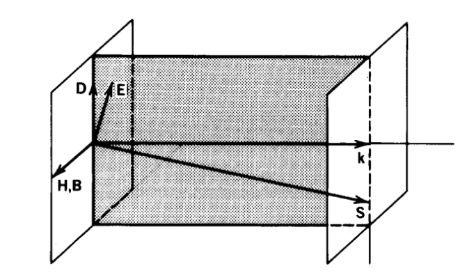
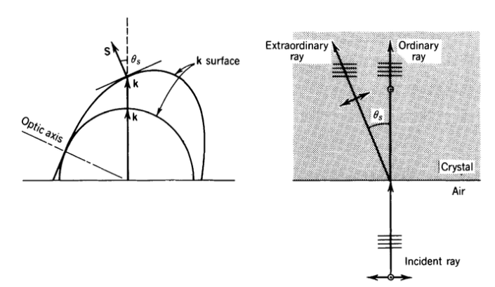
Energy flow vs. phase propagation divergence: Since D and E are not parallel, the Poynting vector \(\mathbf{S} = \mathbf{E} \times \mathbf{H}\) (energy flow direction) is no longer parallel to the wave vector k (phase propagation direction). This is most pronounced for the extraordinary ray.
Polarization-dependent propagation: Each mode has a specific polarization state that depends on both the propagation direction and the crystal’s optical properties.
The Extraordinary Ray Phenomenon: The most striking consequence is that the extraordinary ray exhibits “walk-off” - its energy propagates in a different direction than its phase fronts advance. This creates the remarkable situation where a beam of light can physically travel at an angle to its own wave fronts, a phenomenon impossible in isotropic media and directly traceable to the non-parallelism of D and E.
Wave Vector vs. Ray Vector: A Critical Distinction
In anisotropic media, we must carefully distinguish between two different directions:
- Wave vector \(\mathbf{k}\): Direction of phase propagation (perpendicular to wavefronts)
- Ray vector \(\mathbf{k}_r\) (or Poynting vector \(\mathbf{S}\)): Direction of energy flow
In isotropic media: \(\mathbf{k} \parallel \mathbf{S}\) - phase and energy travel in the same direction.
In anisotropic media: \(\mathbf{k} \not\parallel \mathbf{S}\) - phase and energy travel in different directions!
Mathematical relationship: From the Poynting vector \(\mathbf{S} = \frac{1}{\mu_0}\mathbf{E} \times \mathbf{H}\) and Maxwell’s equations:
\[\mathbf{S} = \frac{c}{2\mu_0\omega}(\mathbf{E} \times \mathbf{B}) = \frac{c}{2\mu_0\omega}(\mathbf{E} \times (\mathbf{k} \times \mathbf{E}))\]
In anisotropic media, this becomes: \[\mathbf{S} \propto \mathbf{E} \times (\mathbf{k} \times \mathbf{D}/\varepsilon_0)\]
Since \(\mathbf{D} = \varepsilon_0 \overleftrightarrow{\varepsilon}_r \mathbf{E}\) and \(\mathbf{D} \not\parallel \mathbf{E}\), the energy flow direction differs from the wave vector direction.
Physical consequence: A light beam entering an anisotropic crystal will have its wavefronts traveling in one direction while the actual light energy travels in a slightly different direction - this is the “walk-off” phenomenon.
Birefringence
Derivation of the Dispersion Relation
From Maxwell’s Equations to Plane Wave Form
We start from the standard Maxwell equations in time domain: \[\nabla \times \mathbf{E} = -\frac{\partial \mathbf{B}}{\partial t} = -\mu_0\frac{\partial \mathbf{H}}{\partial t}\] \[\nabla \times \mathbf{H} = \frac{\partial \mathbf{D}}{\partial t}\]
For plane waves with harmonic time dependence \(\mathbf{E}(\mathbf{r},t) = \mathbf{E}(\mathbf{r})e^{-i\omega t}\) and \(\mathbf{H}(\mathbf{r},t) = \mathbf{H}(\mathbf{r})e^{-i\omega t}\): - Time derivatives: \(\frac{\partial}{\partial t} \rightarrow -i\omega\) - Spatial derivatives for plane waves \(e^{i\mathbf{k} \cdot \mathbf{r}}\): \(\nabla \rightarrow i\mathbf{k}\)
This transforms Maxwell’s equations to: \[i\mathbf{k} \times \mathbf{E} = -\mu_0(-i\omega)\mathbf{H} = i\omega\mu_0\mathbf{H}\] \[i\mathbf{k} \times \mathbf{H} = (-i\omega)\mathbf{D} = -i\omega\mathbf{D}\]
Dividing by \(i\) gives us the frequency domain plane wave Maxwell equations:
\[\mathbf{k} \times \mathbf{E} = \omega \mu_0 \mathbf{H}\] \[\mathbf{k} \times \mathbf{H} = -\omega \mathbf{D}\]
We can derive the fundamental wave equation for anisotropic media. Taking the cross product of the first equation with k:
\[\mathbf{k} \times (\mathbf{k} \times \mathbf{E}) = \omega \mu_0 (\mathbf{k} \times \mathbf{H})\]
Using the vector identity \(\mathbf{k} \times (\mathbf{k} \times \mathbf{E}) = \mathbf{k}(\mathbf{k} \cdot \mathbf{E}) - k^2\mathbf{E}\) and substituting the second Maxwell equation:
\[\mathbf{k}(\mathbf{k} \cdot \mathbf{E}) - k^2\mathbf{E} = \omega \mu_0(-\omega \mathbf{D}) = -\omega^2 \mu_0 \mathbf{D}\]
Rearranging: \[k^2\mathbf{E} - \mathbf{k}(\mathbf{k} \cdot \mathbf{E}) = \omega^2 \mu_0 \mathbf{D}\]
Substituting the constitutive relation \(\mathbf{D} = \varepsilon_0 \overleftrightarrow{\varepsilon}_r \mathbf{E}\) and using \(c^2 = 1/(\mu_0 \varepsilon_0)\):
\[k^2\mathbf{E} - \mathbf{k}(\mathbf{k} \cdot \mathbf{E}) = \frac{\omega^2}{c^2} \overleftrightarrow{\varepsilon}_r \mathbf{E}\]
This is the fundamental wave equation in anisotropic media.
Component Form and the Fresnel Equation
Let’s work in the principal axes coordinate system where the permittivity tensor is diagonal:
\[\overleftrightarrow{\varepsilon}_r = \begin{pmatrix} n_x^2 & 0 & 0 \\ 0 & n_y^2 & 0 \\ 0 & 0 & n_z^2 \end{pmatrix}\]
Let \(\mathbf{k} = k(\sin\theta\cos\phi, \sin\theta\sin\phi, \cos\theta)\) and define the refractive index \(n = ck/\omega\). The wave equation becomes:
\[n^2\mathbf{E} - \mathbf{\hat{k}}(\mathbf{\hat{k}} \cdot \mathbf{E}) = \overleftrightarrow{\varepsilon}_r \mathbf{E}\]
where \(\mathbf{\hat{k}} = \mathbf{k}/k\) is the unit wave vector.
In component form: \[\left(n^2 - \hat{k}_x^2\right)E_x - \hat{k}_x\hat{k}_yE_y - \hat{k}_x\hat{k}_zE_z = n_x^2E_x\] \[-\hat{k}_y\hat{k}_xE_x + \left(n^2 - \hat{k}_y^2\right)E_y - \hat{k}_y\hat{k}_zE_z = n_y^2E_y\] \[-\hat{k}_z\hat{k}_xE_x - \hat{k}_z\hat{k}_yE_y + \left(n^2 - \hat{k}_z^2\right)E_z = n_z^2E_z\]
Rearranging into matrix form and using \(\hat{k}_x^2 + \hat{k}_y^2 + \hat{k}_z^2 = 1\): \[\begin{pmatrix} n^2(\hat{k}_y^2 + \hat{k}_z^2) - n_x^2 & -n^2\hat{k}_x\hat{k}_y & -n^2\hat{k}_x\hat{k}_z \\ -n^2\hat{k}_y\hat{k}_x & n^2(\hat{k}_x^2 + \hat{k}_z^2) - n_y^2 & -n^2\hat{k}_y\hat{k}_z \\ -n^2\hat{k}_z\hat{k}_x & -n^2\hat{k}_z\hat{k}_y & n^2(\hat{k}_x^2 + \hat{k}_y^2) - n_z^2 \end{pmatrix}\begin{pmatrix} E_x \\ E_y \\ E_z \end{pmatrix} = \begin{pmatrix} 0 \\ 0 \\ 0 \end{pmatrix}\]
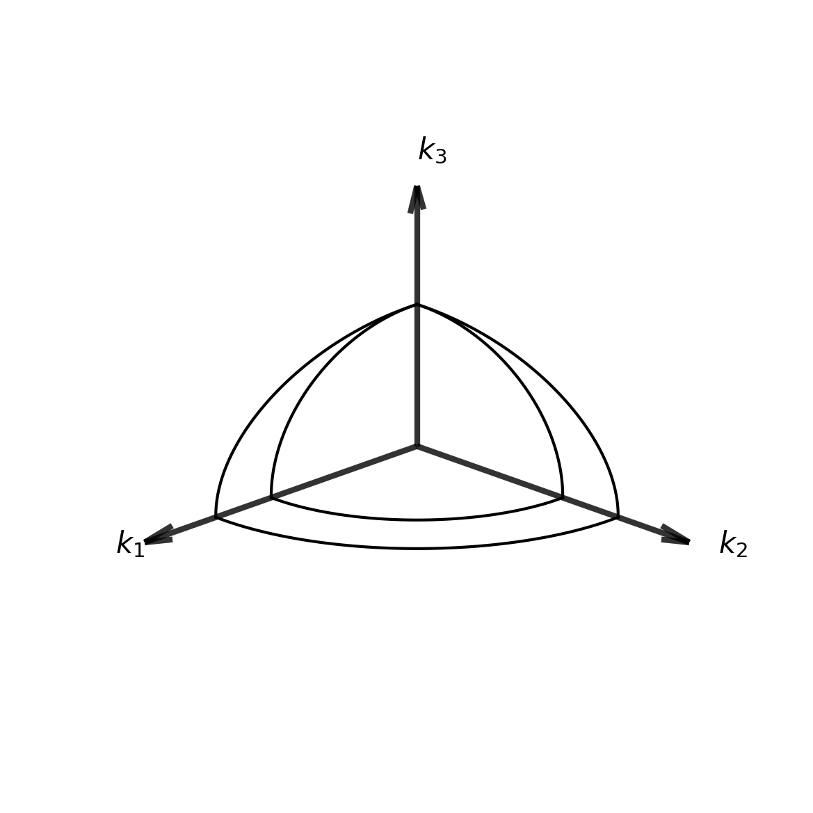
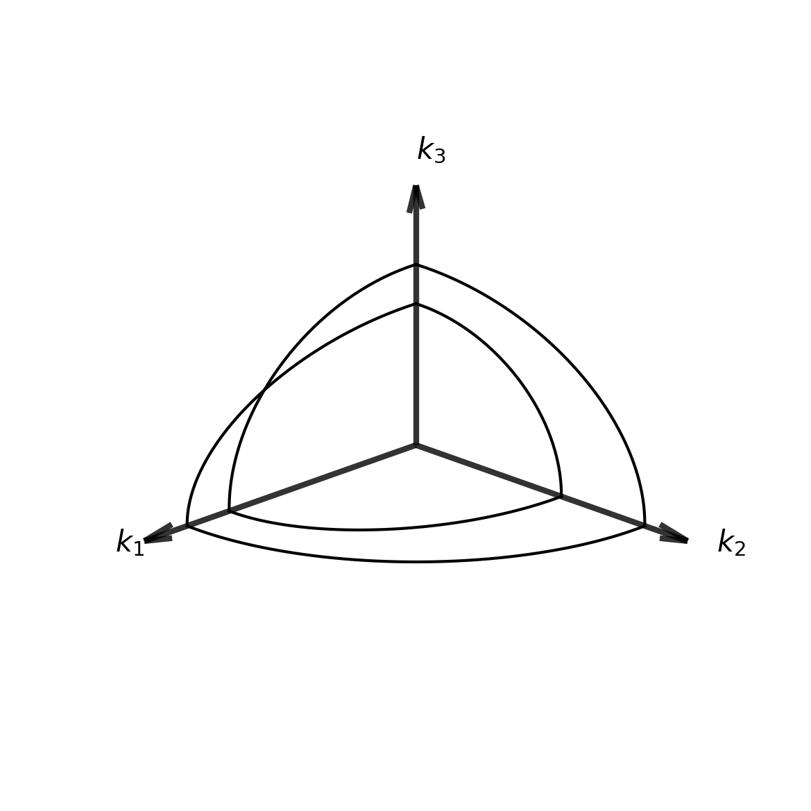
For non-trivial solutions, the determinant must be zero, yielding Fresnel’s wave surface equation:
\[\det\begin{pmatrix} n^2(\hat{k}_y^2 + \hat{k}_z^2) - n_x^2 & -n^2\hat{k}_x\hat{k}_y & -n^2\hat{k}_x\hat{k}_z \\ -n^2\hat{k}_y\hat{k}_x & n^2(\hat{k}_x^2 + \hat{k}_z^2) - n_y^2 & -n^2\hat{k}_y\hat{k}_z \\ -n^2\hat{k}_z\hat{k}_x & -n^2\hat{k}_z\hat{k}_y & n^2(\hat{k}_x^2 + \hat{k}_y^2) - n_z^2 \end{pmatrix} = 0\]
This is a quartic equation in \(n^2\), generally yielding four solutions (two pairs of \(\pm n\)), corresponding to two distinct modes of propagation.
Terminology Note
This determinant equation is called the Fresnel equation (or Fresnel’s wave surface equation) in crystal optics. This should not be confused with the more commonly known Fresnel equations for reflection and transmission coefficients at interfaces (which give \(r_s\), \(r_p\), \(t_s\), \(t_p\)). Both are named after Augustin-Jean Fresnel, but they describe completely different physical phenomena:
- Fresnel’s wave surface equation (shown above): Determines allowed refractive indices for wave propagation in anisotropic crystals
- Fresnel reflection/transmission equations: Determine amplitude coefficients for reflection and transmission at optical interfaces
The terminology overlap is historical and can be confusing, but both are standard usage in optics literature.
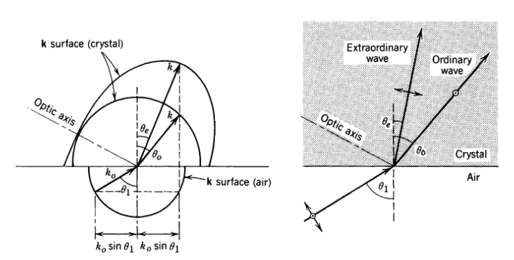
Uniaxial Crystals: Special Case Analysis
Definition and Properties
Uniaxial crystals occur when two principal refractive indices are equal: \[n_x = n_y = n_o \text{ (ordinary index)}, \quad n_z = n_e \text{ (extraordinary index)}\]
The \(z\)-axis is called the optical axis.
Simplification of Fresnel’s Wave Surface Equation
For uniaxial crystals, let’s consider propagation at angle \(\theta\) to the optical axis (\(\phi = 0\) for simplicity): \[\mathbf{\hat{k}} = (\sin\theta, 0, \cos\theta)\]
Fresnel’s wave surface equation becomes: \[\det\begin{pmatrix} n^2 - n_o^2 - \sin^2\theta & 0 & -\sin\theta\cos\theta \\ 0 & n^2 - n_o^2 & 0 \\ -\sin\theta\cos\theta & 0 & n^2 - n_e^2 - \cos^2\theta \end{pmatrix} = 0\]
This factors as: \[(n^2 - n_o^2)\left[(n^2 - n_o^2 - \sin^2\theta)(n^2 - n_e^2 - \cos^2\theta) - \sin^2\theta\cos^2\theta\right] = 0\]
Two Distinct Solutions
Solution 1 (Ordinary Ray): \[n^2 = n_o^2\]
This gives \(n = n_o\) independent of propagation direction \(\theta\).
Solution 2 (Extraordinary Ray): From the remaining factor: \[(n^2 - n_o^2 - \sin^2\theta)(n^2 - n_e^2 - \cos^2\theta) = \sin^2\theta\cos^2\theta\]
Expanding and simplifying: \[n^4 - n^2(n_o^2 + n_e^2 + 1) + n_o^2n_e^2 + n_o^2\cos^2\theta + n_e^2\sin^2\theta = 0\]
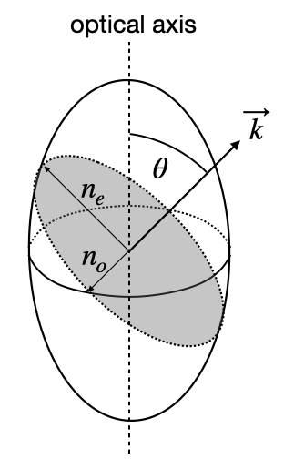
After algebraic manipulation, this yields: \[\frac{1}{n_e^2(\theta)} = \frac{\sin^2\theta}{n_e^2} + \frac{\cos^2\theta}{n_o^2}\]
where \(\theta\) is the angle between the wave vector k and the optical axis (z-direction), and \(n_e\), \(n_o\) are the principal extraordinary and ordinary indices respectively.
Key points:
- For \(\theta = 0°\) (propagation along optic axis): \(n_e(\theta) = n_o\)
- For \(\theta = 90°\) (propagation perpendicular to optic axis): \(n_e(\theta) = n_e\)
- This formula applies only to uniaxial crystals in the principal axis coordinate system
Classification of Uniaxial Crystals
- Positive uniaxial: \(n_e > n_o\) (e.g., quartz, \(n_o = 1.544\), \(n_e = 1.553\))
- Negative uniaxial: \(n_e < n_o\) (e.g., calcite, \(n_o = 1.658\), \(n_e = 1.486\))
Biaxial Crystals: General Case
Definition and Properties
Biaxial crystals have three distinct principal refractive indices: \[n_x \neq n_y \neq n_z\]
The ordering convention is typically \(n_x < n_y < n_z\), where: - \(n_x\) = smallest refractive index (α-axis) - \(n_y\) = intermediate refractive index (β-axis) - \(n_z\) = largest refractive index (γ-axis)
Unlike uniaxial crystals with one optical axis, biaxial crystals have two optical axes.
Simplification of the Fresnel Equation
For biaxial crystals, consider propagation in the \(xz\)-plane (\(\phi = 0\)) at angle \(\theta\) to the \(z\)-axis: \[\mathbf{\hat{k}} = (\sin\theta, 0, \cos\theta)\]
The Fresnel equation becomes: \[\det\begin{pmatrix} n^2 - n_x^2 - \sin^2\theta & 0 & -\sin\theta\cos\theta \\ 0 & n^2 - n_y^2 & 0 \\ -\sin\theta\cos\theta & 0 & n^2 - n_z^2 - \cos^2\theta \end{pmatrix} = 0\]
This factors as: \[(n^2 - n_y^2)\left[(n^2 - n_x^2 - \sin^2\theta)(n^2 - n_z^2 - \cos^2\theta) - \sin^2\theta\cos^2\theta\right] = 0\]
Two Distinct Solutions
Solution 1 (β-ray): \[n^2 = n_y^2\]
This gives \(n = n_y\) independent of propagation direction \(\theta\) when propagating in the \(xz\)-plane.
Solution 2 (αγ-ray): From the remaining factor: \[(n^2 - n_x^2 - \sin^2\theta)(n^2 - n_z^2 - \cos^2\theta) = \sin^2\theta\cos^2\theta\]
Expanding and solving this quadratic equation in \(n^2\): \[n^4 - n^2(n_x^2 + n_z^2 + 1) + n_x^2n_z^2 + n_x^2\cos^2\theta + n_z^2\sin^2\theta = 0\]
This yields the biaxial dispersion relation: \[\frac{1}{n^2} = \frac{\cos^2\theta}{n_x^2} + \frac{\sin^2\theta}{n_z^2}\]
for propagation in the \(xz\)-plane, where \(\theta\) is the angle between the wave vector k and the \(z\)-axis.
Key points:
- For \(\theta = 0°\) (propagation along \(z\)-axis): \(n = n_x\)
- For \(\theta = 90°\) (propagation along \(x\)-axis): \(n = n_z\)
- The optical axes occur at angles where the two solutions become equal
Classification of Biaxial Crystals
Biaxial crystals have two optical axes located symmetrically about the intermediate refractive index axis. The angle between these optical axes is called the optic angle \(2V\).
The optical axes are located at angles \(\pm V\) from the \(z\)-axis, where: \[\cos^2 V = \frac{n_y^2 - n_x^2}{n_z^2 - n_x^2}\]
Optical sign classification:
- Positive biaxial: \(2V < 90°\) (small optic angle)
- Negative biaxial: \(2V > 90°\) (large optic angle)
Examples:
- Positive biaxial: Topaz, Mica (small angle between optical axes)
- Negative biaxial: Gypsum, Aragonite (large angle between optical axes)
The distinction between positive and negative biaxial crystals is important for optical applications and crystal identification.
Applications
Wave Plates
Wave plates (retarders) are birefringent crystals of controlled thickness that introduce precise phase differences between orthogonal polarization components. Let’s analyze how a linearly polarized wave is modified as it propagates through these crystals.
Input Wave Analysis: Consider a linearly polarized wave entering a wave plate:
\[\mathbf{E}_{input} = E_0(\cos\alpha \hat{\mathbf{f}} + \sin\alpha \hat{\mathbf{s}})e^{i(kz-\omega t)}\]
In this expression, \(\hat{\mathbf{f}}\) and \(\hat{\mathbf{s}}\) represent unit vectors along the crystal’s fast and slow axes respectively, while \(\alpha\) denotes the angle between the input polarization and the fast axis, and \(E_0\) is the amplitude of the electric field.
Propagation Through Crystal: As the wave propagates through the crystal of thickness \(d\), each polarization component experiences a different refractive index. The component along the fast axis evolves as \(E_f = E_0\cos\alpha \cdot e^{i(k_f z - \omega t)}\) where \(k_f = \frac{2\pi n_f}{\lambda}\), while the slow axis component propagates as \(E_s = E_0\sin\alpha \cdot e^{i(k_s z - \omega t)}\) where \(k_s = \frac{2\pi n_s}{\lambda}\). This differential propagation is the fundamental mechanism that enables wave plates to manipulate polarization states.
After propagating through thickness \(d\), the wave becomes:
\[\mathbf{E}_{output} = E_0\cos\alpha \cdot e^{i(k_f d - \omega t)}\hat{\mathbf{f}} + E_0\sin\alpha \cdot e^{i(k_s d - \omega t)}\hat{\mathbf{s}}\]
Phase Difference: The crucial parameter is the phase difference (retardance) acquired between the two components:
\[\delta = (k_s - k_f)d = \frac{2\pi d}{\lambda}(n_s - n_f) = \frac{2\pi d}{\lambda}|n_e - n_o|\]
Output Wave: Factoring out the common phase term:
\[\mathbf{E}_{output} = E_0 e^{i(k_f d - \omega t)}[\cos\alpha \hat{\mathbf{f}} + \sin\alpha \cdot e^{i\delta}\hat{\mathbf{s}}]\]
The relative phase shift \(e^{i\delta}\) between the components determines the output polarization state.
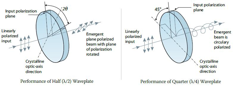
Quarter-Wave Plate
A quarter-wave plate is designed to introduce a phase difference of \(\delta = \pi/2\) between orthogonal polarization components, requiring a thickness of \(d = \frac{\lambda}{4|n_e - n_o|}\). This specific phase relationship enables the conversion between linear and circular polarization states.
Polarization transformation: For \(\alpha = 45°\) (input at 45° to crystal axes): \[\mathbf{E}_{output} = \frac{E_0}{\sqrt{2}} e^{i(k_f d - \omega t)}[\hat{\mathbf{f}} + e^{i\pi/2}\hat{\mathbf{s}}] = \frac{E_0}{\sqrt{2}} e^{i(k_f d - \omega t)}[\hat{\mathbf{f}} + i\hat{\mathbf{s}}]\]
This represents circularly polarized light since the two orthogonal components have equal amplitudes and are 90° out of phase.
For arbitrary input angle \(\alpha\), the output becomes: \[\mathbf{E}_{output} = E_0 e^{i(k_f d - \omega t)}[\cos\alpha \hat{\mathbf{f}} + i\sin\alpha \hat{\mathbf{s}}]\]
This produces elliptically polarized light with ellipticity determined by \(\alpha\). The quarter-wave plate thus provides complete control over the conversion from linear to circular or elliptical polarization, making it essential for applications requiring specific polarization states.
Half-Wave Plate
A half-wave plate introduces a phase difference of \(\delta = \pi\) between orthogonal components, achieved with a thickness of \(d = \frac{\lambda}{2|n_e - n_o|}\). This design creates a fundamentally different polarization transformation compared to the quarter-wave plate.
Polarization transformation: \[\mathbf{E}_{output} = E_0 e^{i(k_f d - \omega t)}[\cos\alpha \hat{\mathbf{f}} + \sin\alpha \cdot e^{i\pi}\hat{\mathbf{s}}] = E_0 e^{i(k_f d - \omega t)}[\cos\alpha \hat{\mathbf{f}} - \sin\alpha \hat{\mathbf{s}}]\]
The key result is that the output remains linearly polarized but is rotated by \(2\alpha\) relative to the input. If the input makes angle \(\alpha\) with the fast axis, the output makes angle \(-\alpha\) with the fast axis, resulting in a total rotation of \(2\alpha\). The \(\pi\) phase shift effectively reverses the slow-axis component, causing the polarization vector to flip across the fast axis, doubling the rotation angle.
These wave plates find extensive applications in modern photonics. Quarter-wave plates enable the conversion between linear and circular or elliptical polarization states, making them crucial for circular dichroism spectroscopy, optical communication systems, and laser applications. Half-wave plates provide precise polarization rotation and linear polarization direction control, essential for optical isolators, variable attenuators, and polarization-sensitive measurement systems.