This page was generated from `/home/lectures/exp3/source/notebooks/L14/EM Waves in Matter.ipynb`_.

Electromagnetic Waves in Matter

So far we have only considered electromagnetic waves in vacuum. We would now like to extend our description of electromagnetic waves to the propagation in materials. Before we do that, we will have a qiuck look the polarisation, i.e. the separation of change centers of atoms by electric fields.

Let us construct a very crude atomic model, where an electronic charge \(q\) is smeared out over a spherical volume of radius \(a\). The charge density of the charge cloud is then given by

\[\rho=\frac{-q}{\frac{4}{3}\pi a^{3}}=-\frac{3q}{4\pi a^3}\]

Inside this charge cloud sits our positive necleus in an electric field

\[E(r)=-\frac{1}{4\pi\epsilon_0}\frac{qr}{a^3}\]

where \(r\) is the distance from the center of the charge cloud. If we now apply an external field to this atom, the postive nucleus will be displaced from the center of the negative cloud by a distance \(d\) from the center such that the external forces on the charges will be belanced by the internal forces between the charge cloud and the nucleus.

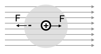
Fig.: Polarization of an electric cloud of an atom.

The external force is given by \(F=qE_{\rm ex}\) and the force balance therefore

\[qE_{\rm ex}-\frac{1}{4\pi\epsilon_0}\frac{q^2d}{a^3}\]

from which we find the distance

\[d=4\pi \epsilon_0 a^3 \frac{E_{\rm ex}}{q}\]

and finally also the dipole moment

\[p=qd=4\pi\epsilon_0 a^3 E_{\rm ex}\]

The dipole moment therefore increases in our crude model linearly with the external field and the slope of this linear increase is given by

\[\alpha=4\pi \epsilon_0 a^3\]

which is known as the electronic polarizability. Note, that the electronic polarizability depends on the volume of the atom here.

In a material with many of those atomic dipoles a chain of dipoles as the first row in the Figure below creates a dipole, which is 4 times the atomic dipole. Overall, for \(N\) dipoles in a volume, we create a dipole density

\[\vec{P}=N\vec{p}\]

which is also known as polatization density. The dipole density is pointing in the same direction as the dipoles, which is from \(-\) to \(+\). If the picture below shows a cylindrical piece of material with a cap of area \(A\) and a height \(s\), then the dipole moment of this cylinder is given by

\[p_{\rm cyl}=A s P\]

The charges which sit at the cylinder caps are therefore given by

\[q_{\rm end}=\frac{p_{\rm cyl}}{s}=A P\]

and therefore the caps charge surface density is

\[\sigma=\frac{q_{\rm end}}{A}=P\]

The surface charge density is therefore given by the polarization density or more generally by

\[\sigma=\vec{P}\hat{n}\]

where \(\hat{n}\) is the surface normal. Thus \(\vec{P}\) and \(\hat{n}\) are anti-parallel on the negative side giving a negative charge and parallel on the positive side giving a positive charge density. These charges appearing at the surface are belonging to atoms. We call those charges bound charges in contrast to free charges. The surface density of bound charges is then \(\sigma_b\).

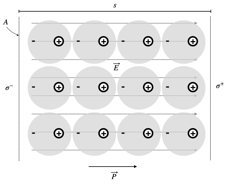
Fig.: Polarization of an electric cloud of an atom.

The above relation between surface charge density and polarisation density is only true if all the induced bound charges inside the material cancel and the is no residual charge density inside the volume. However, if the surfaces charges on both ends of the cap are not equal and no excess charges present, there must be a volume charge inside the material, which creates a volume charge density of bound charges \(\rho_b\). Thus in general we have

\[\int \sigma_b dA +\int \rho_b dv=0\]

which we can transform with Gauss theorem to

\[\int \rho_b dv=-\int \sigma_b dA =-\int \vec{P}d\vec{A}\]

and thus finally to

\[\rho_b=-\nabla\cdot \vec{P}\]

which states, that the sources of the polarisation density are the bound charges induced in the volume.

The divergence of the total electric field with free charges in vacuum was given by

\[\nabla \cdot \vec{E}=\frac{\rho}{\epsilon_0}\]

where the charge density in vaucuum refers to free chrages that are not bound to atoms. In a material we now also have to consider the boundar charges, which create the polarisation density and therefore

\[\nabla \cdot \vec{E}=\frac{\rho_{\rm f}+\rho_{\rm b}}{\epsilon_0}\]

where \(\rho_f\) refers to the free charges. Inserting now \(\rho_b=-\nabla\cdot \vec{P}\), we can rewrite this Maxwell equation as

\[\nabla \cdot(\epsilon_0\vec{E}+\vec{P})=\rho_f\]

The term in the parenthesis can now be defined as a new quantity, for which the original equation (divergence of the electric field is the free charge density) is valid again. This quantity is the displacement field \(\vec{D}\)

\[\vec{D}=\epsilon_0 \vec{E}+\vec{P}\]

for which

\[\nabla \cdot \vec{D} =\rho_f\]

is valid.

Dielectrics Polarization

Based on our previous findings of the dipole density and its dependence on the exlectric field \(\vec{E}\), we can also write down

\[\vec{P}=\epsilon_0\chi\vec{E}\]

where we introduced a response function, which is the electronic sucesptibility \(\chi\). Since the relation between \(\vec{P}\) and \(\vec{E}\) is linear, we call those materials linear materials. Remember, that this linearity is based on the crude atomic model we introduced. In general, this is not true and materials have a nonlinear response to external electric fields. These nonlinearities are subject of the field nonlinear optics.

Within the linear approximation we can now express the displacement field also via the susceptibility \(\chi\) or even a new quantity \(\epsilon\), which is the electronic permittivity.

\[\vec{D}=\epsilon_0 \vec{E}+\vec{P}=\epsilon_0 (1+\chi)\vec{E}=\epsilon \vec{E}\]

with

\[\epsilon=\epsilon_0 (1+\chi) \tag{electronic permittivity}\]

The ratio

\[\frac{\epsilon}{\epsilon_0}=1+\chi=\epsilon_r\]

is called the dielectric constant, even though this number is a function of the frequency of the electromagnetic field. The dielectric function is a material property, which describes the interacion of electric fields with the dielectric material and thus also the interaction with of dielectrics with electromagnetic waves.

Magnetization

Similar arguments as before can also be made for magnetic materials even though there are no free magnetic monopoles. For completeness we provide a relation between the magnetic flux density \(\vec{B}\) and the magnetic field \(\vec{H}\) here.

The flux density \(\vec{B}\) is related to the magnetic field by

\[\vec{B}=\mu_0(1+\chi_m)\vec{H}\]

where \(\chi_m\) is the magnetic susceptibility.

The quantity equivalent to the polarization density is the magnetization \(\vec{M}\)

\[\frac{1}{\mu_0}\vec{B}=\vec{H}+\vec{M}\]

which is the density of the magnetic dipole moments.

Maxwell Equations in Matter

We can now write down the Maxwell equation in Matter including possible charges as well as currents.

\[\nabla \times \vec{E}=-\frac{\partial \vec{B}}{\partial t} \label{eq:ME1}\tag{ME.1}\]

\[\nabla\cdot\vec{D}=\rho_f \tag{ME.2}\]

\[\nabla\times \vec{H}=\frac{\partial \vec{D}}{\partial t}+\vec{j}_f \tag{ME.3}\]

\[\nabla\cdot \vec{B}=0 \tag{ME.4}\]

Here \(\vec{j}_f\) is the current density of free charges and \(\rho_f\) resembles the free charge density. In case of an insulator with no free charges both quantities are zero.

In addition, we have the electric displacement field \(\vec{D}=\epsilon \vec{E}\) and the magnetic flux density \(\vec{B}=\mu \vec{H}\), where the material coefficients are given by

\begin{eqnarray} \epsilon&=&\epsilon_0 \epsilon_r\\ \mu&=&\mu_0 \mu_r\\ \end{eqnarray}

Wave Equation and Refractive Index

Applying the same procedure as during the derivation of the wave equation, we can get the wave equation in matter for \(\vec{j}_f=0\) and \(\rho_f=0\), which reads

\[\frac{\partial^2 \vec{E}}{\partial \vec{r}^2}-\frac{1}{v^2} \frac{\partial^2\vec{E}}{\partial t^2}=0\]

where \(v\) is the speed of light in the medium. This phase velocity is now given by

\[v^2=\frac{c^2}{\epsilon_r\mu_r}\]

or

\[v=\frac{1}{\sqrt{\epsilon_0 \mu_0}}\frac{1}{\sqrt{\epsilon_r\mu_r}}=\frac{c}{\sqrt{\epsilon_r\mu_r}}\]

The speed of light in a medium is thus reduced by a factor \(\sqrt{\epsilon_r\mu_r}\) as compared to the speed of light in vacuum \(c\). For non-magnetic materials, the magnetic permeability is \(\mu_r=1\) and we have

\[\frac{c}{v}=\sqrt{\epsilon_r}=n \tag{refractive index}\]

which provides us with a definition of the refractive index \(n\). As we have walked our way from the polarization of a single atom in an electric field via bound charges to the dielectric function \(\epsilon_r\), we now know that the refractive index is the result of the polarizability of atoms.

The refractive index is commonly found to be \(n\ge1\) for common materials. However, as the square of the phase velocity in the material is defined as \(v^2=\frac{c^2}{\epsilon_r\mu_r}\), i.e. by the product of \(\epsilon_r\mu_r\), the solution is in general given by

\[v=\pm\frac{c}{\sqrt{\epsilon_r\mu_r}} \tag{general phase velocity}\]

and it turns out that

\[v=-\frac{c}{\sqrt{\epsilon_r\mu_r}} \tag{negative refraction}\]

must be selected if \(\mu_r<0\) and \(\epsilon_r<0\). In this case, the refractive index is negative which leads to a number of exciting possibilities. Materials, which have such unusual refractive properties need to be designed in a specific way since they also need to have specific magnetic properties. Such materials belong to the field of meta-materials as they include smaller subunits that are specifically arranged.

We can no insert the solution of a monochromatic plane wave

\[\vec{E}=\vec{E}_0e^{i(\omega t- \vec{k}\cdot \vec{r})}\]

into the wave equation, which yields

\[k^{2}=\frac{\omega^2}{v^2}=0\]

from which we find

\[k=\frac{\omega}{v}\]

which finally leads to

\[\vec{k}=n\vec{k}_0\]

where \(\vec{k}_0\) is the wavevector in vacuum.