This page was generated from `/home/lectures/exp3/source/notebooks/L25_AMA/L25_Schroedinger_equation.ipynb`_.

The Schrödinger Equation

Introducing the equation

First we discuss the simple case of a free particle with mass \(m\) at uniform motion with velocity \(u\) along the \(x\) direction. We set the motion at a constant potential (\(E_{\mathrm{pot}} = 0\)) and get a matter wave like

\[\psi \left(x,t\right) = A \cdot \mathrm{e}^{i\left( k x - \omega t\right)} = A \cdot \mathrm{e}^{\frac{i}{\hbar}\left(p x - E t\right)} \mathrm{,}\]

whith \(E = E_{\mathrm{kin}} = \hbar \cdot \omega\) and \(p = \hbar \cdot k\). Because the formula is analogue with an electromagnetic wave, we use the same formula as for an electromagnetic wave propagating with a phase velocity of \(u\) along \(x\),

\[\frac{\partial^2 \psi}{\partial x^2} - \frac{1}{u^2} \frac{\partial^2 \psi}{\partial t^2} = 0 \mathrm{.}\]

In order to describe stationary quantum states, namly the momentum \(p\) and enegery \(E\) do not depent on time, we are seeking for a stationary solution of the above equation. Since they are indepent of time, we can write the genernal solution for the wave equation \(\psi \left(x,t\right)\) as a product of a position-dependent factor \(\mathrm{e}^{+ikx}\) and a time-dependent phase \(\mathrm{e}^{-i \omega t}\), such like

\[\begin{split}\begin{eqnarray} \psi \left(x,t\right) & = & A \cdot \mathrm{e}^{i k x} \cdot \mathrm{e}^{-i \omega t}\\ {} & = & \psi \left(x\right) \cdot \mathrm{e}^{-i \omega t}\mathrm{.} \end{eqnarray}\end{split}\]

If we now use this ansatz in the wave equation, we obtain for the derivative in space

\[\frac{\partial^2 \psi}{\partial x^2} = -k^2 \psi = - \frac{p^2}{\hbar^2} \psi = - \frac{2 m}{\hbar^2} E_{\mathrm{kin}} \psi \mathrm{.}\]

In the general case our particle might move within a force field. If it is a conservative field, we can assign a potential energy \(E_{\mathrm{pot}}\) to every point in space keeping the total energy constant \(E = E_{\mathrm{kin}} + E_{\mathrm{pot}}\). Then, we directly obtain the one-dimension stationary Schrödinger equation

\[- \frac{\hbar^2}{2 m} \, \frac{\partial^2 \psi}{\partial x^2} + E_{\mathrm{pot}} \psi = E \psi\]

In the case of a three-dimensional motion of our particle we can analogously use the three-dimensional wave equation,

\[\Delta \psi- \frac{1}{u^2} \frac{\partial^2 \psi}{\partial t^2} = 0 \mathrm{,}\]

and an ansatz in three dimensions,

\[\psi \left(x,y,z,t\right) = \psi \left(x,y,z\right) \cdot \mathrm{e}^{-i \omega t} \mathrm{,}\]

in order to obtain the three-dimensional stationary Schrödinger equation

\[- \frac{\hbar^2}{2 m} \, \Delta \psi + E_{\mathrm{pot}} \psi = E \psi \mathrm{.}\]

If we, in addition, calculate the first order derivative of our matter wave with respect to time, we obtain (for \(E_{\mathrm{pot}} = 0\))

\[\frac{\partial \psi}{\partial t} = - \frac{i}{\hbar} E_{\mathrm{kin}} \, \psi \mathrm{.}\]

In the case of a free particle, the condition \(E_{\mathrm{pot}} = 0\) implies \(E_{\mathrm{kin}} = \; \mathrm{const.}\) and we can combine the derivative in space and in time in order to derive this three-dimensionsial time-dependent equation

\[- \frac{\hbar^2}{2 m} \, \Delta \psi = i \hbar \frac{\partial \psi}{\partial t} \mathrm{.}\]

Please note, in the case of non-stationary problems, namely where \(E = E \left( t \right)\) and \(p = p \left( t \right)\), the simple derivative \(\partial^2 \psi / \partial t^2 = - \omega^2 \psi\) does not hold true anymore and more time-dependent parameters have to be considered. However, Schrödinger proposed for a time-dependent potential energy \(E_{\mathrm{pot}} = E_{\mathrm{pot}} \left(r, t \right)\) the equation

\[- \frac{\hbar^2}{2 m} \, \Delta \psi\left(r, t \right) + E_{\mathrm{pot}} \left(r, t \right) \psi\left(r, t \right) = i \hbar \frac{\partial}{\partial t} \psi\left(r, t \right) \mathrm{,}\]

which was confirmed by numerous experiments. For stationary problems, one can again separate the wave function into a position- and a time-dependent factor and get the stationary Schrödinger equation as stated above.

A potential barrier

The free particle with \(E_{\mathrm{pot}} = 0\) as we discussed it previously might propagate in \(+x\) direction and enter a region with a different potential \(\phi \left( x \ge 0 \right) =\phi_0 > 0\). Thus, the particle experiences a shift in its potential energy from \(E_{\mathrm{pot}} = 0\) for \(x < 0\) to \(E_{\mathrm{pot}} = E_0\) for \(x \ge 0\). This scenario is similar to a light wave at the air-glass interface.

In order to solve the Schrödinger equation for this problem, we split the space \(-\infty < x < \infty\) into two regions. In region 1, where \(E_{\mathrm{pot}} = 0\), we can state the general solution for the one-dimensional stationary Schrödinger equation as

\[- \frac{\hbar^2}{2m} \frac{\partial^2}{\partial x^2} \psi\left( x \right) + E_{\mathrm{pot}} \psi\left( x \right) = E \psi \left( x \right) \mathrm{.}\]

Because \(E_{\mathrm{pot}} = 0\) and \(E = E_{\mathrm{kin}} + E_{\mathrm{pot}}\), we can simplify \(E = E_{\mathrm{kin}} = p^2/\left( 2 m \right) = \hbar^2 k^2 / 2 m\) and get

\[\begin{split}\begin{eqnarray} - \frac{\hbar^2}{2m} \frac{\partial^2}{\partial x^2} \psi\left( x \right) & = & \frac{\hbar^2 k^2}{2 m} \psi \left( x \right)\\ \rightarrow \frac{\partial^2}{\partial x^2} \psi\left( x \right) & = & - k^2 \psi \left( x \right) \mathrm{.} \end{eqnarray}\end{split}\]

The general solution of \(\psi\left( x \right)\) has the shape

\[\psi\left( x \right) = A \cdot \mathrm{e}^{+i k x} + B \cdot \mathrm{e}^{-i k x}\]

and the time-dependent solution for the wave function

\[\begin{split}\begin{eqnarray} \psi \left( x,t \right) & = & \psi \left( x \right) \cdot \mathrm{e}^{-i \omega t}\\ {} & = & A \cdot \mathrm{e}^{i \left( k x - \omega t \right)} + B \cdot \mathrm{e}^{-i \left( k x + \omega t \right)} \end{eqnarray}\end{split}\]

is a superposition of a plane wave propagating in \(+x\) direction and a plane wave propagating in \(-x\) direction. Here, the wave with coefficient \(A\) in propagation along \(+x\) direction and the wave with the coefficient \(B\) is propagation along the \(-x\) direction. The coefficients \(A\) and \(B\) are the amplitudes of both waves and are determined on the basis of boundary conditions. If we now concentrate again on our potantial barrier, we can state for the position-dependent solution in region 1

\[\psi_{\mathrm{1}} \left( x \right) = A \cdot \mathrm{e}^{+i k x} + B \cdot \mathrm{e}^{-i k x} \mathrm{.}\]

For region 2 where \(E_{\mathrm{pot}} = E_0\) we can state the Schrödinger equation as follows

\[\begin{split}\begin{eqnarray} - \frac{\hbar^2}{2m} \frac{\partial^2}{\partial x^2} \psi\left( x \right) + E_0 \psi\left( x \right) & = & E \psi \left( x \right) \\ \rightarrow \frac{\partial^2}{\partial x^2} \psi\left( x \right) - \frac{2m}{\hbar^2} \left(E_0 - E \right) \psi\left( x \right) & = & 0\\ \frac{\partial^2}{\partial x^2} \psi\left( x \right) - \alpha^2 \psi\left( x \right) & = & 0\mathrm{,} \end{eqnarray}\end{split}\]

with \(\alpha = \sqrt{2m\left(E_0 - E \right)}/\hbar\). The solution for region 2 then reads as

\[\psi_{\mathrm{2}} \left( x \right) = C \cdot \mathrm{e}^{+\alpha x} + D \cdot \mathrm{e}^{-\alpha x}\]

and the general solution for the position-dependent factor of the one-dimensional stationary Schrödinger equation reads as

\[\begin{split}\psi \left( x \right) = \begin{cases} \psi_{\mathrm{1}} \left( x \right) & \text{, if $x < 0$}\\ \psi_{\mathrm{2}} \left( x \right) & \text{, if $x \ge 0$} \end{cases} \mathrm{.}\end{split}\]

The general solution does represent a solution of the Schrödinger equation for the whole space \(- \infty < x < \infty\) if and only if \(\psi \left( x \right)\) is continuously differentiable over the whole space. Otherwise the second derivative $ \partial`^2 :nbsphinx-math:psi`:nbsphinx-math:left`( x :nbsphinx-math:right`) / \partial `x^2$ in the Schrödinger equation will be undefined. From this prerequisite the boundary conditions at :math:`x = 0 directly follow,

\[\begin{split}\begin{eqnarray} \psi_{\mathrm{1}} \left( x = 0 \right) & = & \psi_{\mathrm{2}} \left( x = 0 \right)\\ \rightarrow A + B & = & C +D \end{eqnarray}\end{split}\]

and

\[\begin{split}\begin{eqnarray} \frac{\partial}{\partial x} \psi_{\mathrm{1}} \left( x = 0 \right) & = & \frac{\partial}{\partial x} \psi_{\mathrm{2}} \left( x = 0 \right)\\ \rightarrow i k \left(A - B \right) & = & \alpha \left( C - D \right) \mathrm{.} \end{eqnarray}\end{split}\]

The case \(E < E_0\)

In the case \(E<E_0\), \(\alpha\) is a real number. Moreover the coefficient \(C\) has to be \(0\), otherwise \(\psi_{\mathrm{2}}\) will approach \(+\infty\) for \(x \longrightarrow +\infty\). From the boundary conditions we get

\[\begin{split}\begin{eqnarray} B & = & \frac{i k + \alpha}{i k - \alpha} A\\ D & = & \frac{2 i k}{i k - \alpha} A \end{eqnarray}\end{split}\]

and thus the wave function in region 1 (\(x < 0\)) reads as

\[\psi_{\mathrm{1}} \left( x \right) = A \left( \mathrm{e}^{+i k x} + \frac{i k + \alpha}{i k - \alpha} \mathrm{e}^{-i k x} \right)\mathrm{.}\]

Because we do know the wave function and its amplitudes, we can calculate the reflection coefficient as the ratio of the squared reflected and initial waves,

\[R = \frac{\left| B \cdot \mathrm{e}^{-i k x} \right|^2}{\left| A \cdot \mathrm{e}^{+i k x} \right|^2} = \frac{\left| B \right|^2}{\left| A \right|^2} = \frac{\left| i k + \alpha \right|^2}{\left| i k - \alpha \right|^2} = 1 \mathrm{.}\]

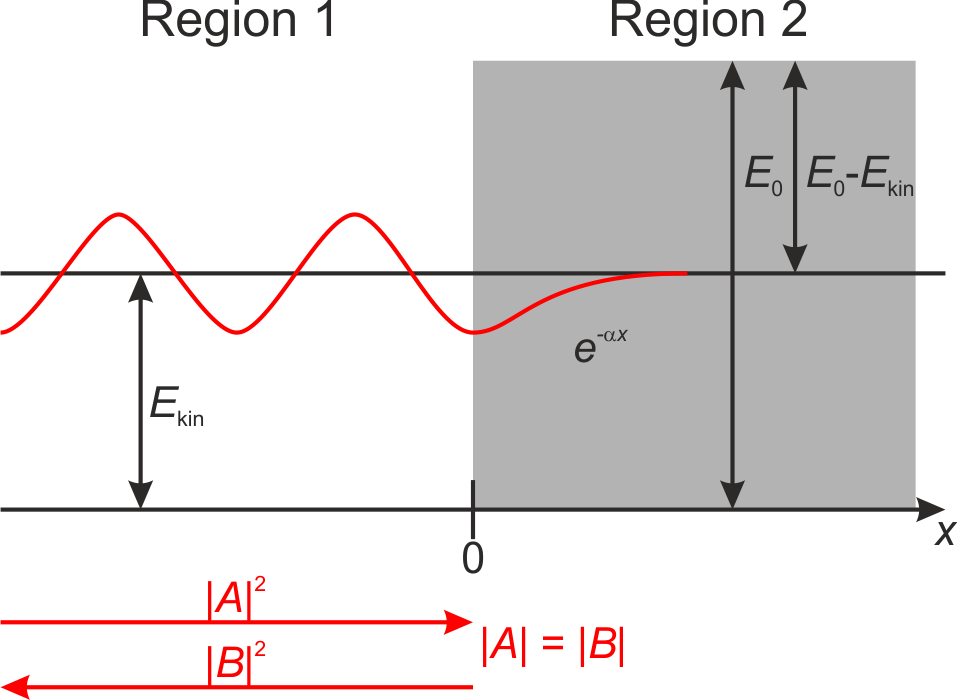
From this result it is evedent that in the case \(E < E_0\) every particle is reflected at the barrier as to be expected in the framework of classical mechanics. However, the particles do not change their direction of propagation diretly at the edge of the barrier (\(x = 0\)). Instead, they are able to intrude into region 2 (\(x \ge 0\)) to some extend, even though their energy is not sufficient ( if discussed in the classical framework).

The probibility density \(P \left( x \right)\) to find a particle at the position \(x\) (with \(x > 0\)) then is given through

\[P \left( x \right) = \left| \psi_2 \left( x \right) \right|^2 = \left| D \cdot \mathrm{e}^{- \alpha x} \right|^2 = \frac{4 k^2}{\alpha^2 + k^2} \mathrm{e}^{-2 \alpha x} = \frac{4 k^2}{k_0^2} \mathrm{e}^{-2 \alpha x} \mathrm{,}\]

where \(k^2 = 2 m E / \hbar^2\) and \(k_0^2 = 2 m E_0 / \hbar^2\). We see, at a depth of penetration of \(x = 1/\left(2\alpha\right)\) the propability density to find the particle at this position is decreased about the fractor \(1/\mathrm{e}\) compared to the propability density at \(x=0\). This phenomenon we allready know as evanescent waves during total internal reflection.

Fig.: A wave with a kinetic energy :math:`E_{mathrm{kin}}` approaches a potential barrier :math:`E_0` with :math:`E_0 > E_{mathrm{kin}}`. The wave is completely reflacted (amplitudes :math:`left|Aright|` = :math:`left|Bright|`), but intrudes the barrier where the amplitude decays exponentially.

The case \(E > E_0\)

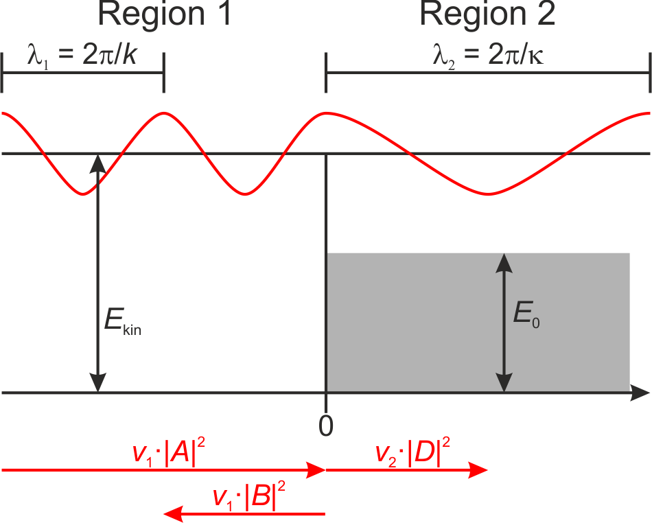
In this case the kinetic energy is greater than the shift in the potential energy. In the framework of classical mechanics, every particle is allowed to enter region 2 (\(x>0\)) and to propagate there, but with a reduced velocity due to their decreased kinetic energy (\(E_{\mathrm{kin}} = E - E_0\)).

In the framwork of matter waves the parameter \(\alpha\) now is an imaginary number. Therefore, we introduce a real number,

\[\kappa = i \alpha = \frac{\sqrt{2 m \left( E - E_0 \right)}}{\hbar} \mathrm{.}\]

The solution for the position-dependent amplitude \(\psi_2 \left( x \right)\) in region 2 then reads as

\[\psi_2 \left( x \right) = C \cdot \mathrm{e}^{-i \kappa x} + D \cdot \mathrm{e}^{+i \kappa x} \mathrm{,}\]

whereas the solution \(\psi_1 \left( x \right)\) for the stationary equation in region 1 remains the same as stated above.

As in the case of the first example, we state the boundary conditions at \(x = 0\) as

\[\begin{split}\begin{eqnarray} \psi_{\mathrm{1}} \left( x = 0 \right) & = & \psi_{\mathrm{2}} \left( x = 0 \right)\\ \rightarrow A + B & = & C +D \end{eqnarray}\end{split}\]

and

\[\begin{split}\begin{eqnarray} \frac{\partial}{\partial x} \psi_{\mathrm{1}} \left( x = 0 \right) & = & \frac{\partial}{\partial x} \psi_{\mathrm{2}} \left( x = 0 \right)\\ \rightarrow i k \left(A - B \right) & = & i \kappa \left( -C + D \right) \mathrm{.} \end{eqnarray}\end{split}\]

Furthermore, in region 2 there is no wave propagating along the \(-x\) direction since there is no boundary located in region 2 in order to reflect the wave. Thus, we can set \(C = 0\). From the boundary conditions it follows

\[\begin{split}\begin{eqnarray} B & = & \frac{k - \kappa}{k + \kappa} A\\ D & = & \frac{2}{k + \kappa} A\\ \end{eqnarray}\end{split}\]

and the wave functions read as

\[\begin{split}\begin{eqnarray} \psi_{\mathrm{1}} \left( x \right) & = & A \left( \mathrm{e}^{+i k x} + \frac{k - \kappa}{ k + \kappa} \mathrm{e}^{-i k x} \right)\\ \psi_{\mathrm{2}} \left( x \right) & = & A \frac{2 k}{ k + \kappa} \mathrm{e}^{+i \kappa x} \mathrm{.} \end{eqnarray}\end{split}\]

For the reflection coefficient it follows

\[R = \frac{\left| B \right|^2}{\left| A \right|^2} = \frac{\left| k - \kappa \right|^2}{\left| k + \kappa \right|^2}\]

and we see, even though the kinetic energy of our pairticle is sufficient enough to overcome the potential barrier, a part of the wave is reflected. Furthermore, since the wavenumber is directly connected to the refrective index \(k = n_1 \cdot k_0\) and \(\kappa = n_2 \cdot k_0\), we can immediately calculate the reflectance,

\[R = \frac{\left| n_1 - n_2 \right|^2}{\left| n_1 + n_2 \right|^2}\mathrm{.}\]

In order to calculate the transmission coefficient, or how many particles pass a unit area at \(x=x_0>0\) per time devided through how many incident particles pass a unit area at \(x=-x_0<0\) per time, we have to bear in mind the different propagation velocities in region 1 and 2. The ratio of the velocities is governed by the ratio of the wavenumbers

\[\frac{v_2}{v_1} = \frac{\lambda_2}{\lambda_1} = \frac{k}{\kappa} \mathrm{.}\]

The transmission coefficient then reads as

\[T = \frac{v_1 \cdot \left| D \right|^2}{v_2 \cdot \left| A \right|^2} = \frac{4 \kappa k}{\left( k + \kappa \right)^2}\mathrm{.}\]

Moreover, it is evident that

\[R + T = 1 \mathrm{,}\]

which represents the conservation of the number of particles. Please note, for the limiting case \(E = E_0\) every exponent becomes \(0\) (\(\alpha = 0\) as well as \(\kappa = 0\)) and the reflection coefficient becomes \(R=1\).

Fig.: A wave with a kinetic energy :math:`E_{mathrm{kin}}` approaches potential barrier :math:`E_0` with $E_{:nbsphinx-math:`mathrm{kin}`} > E_0 $. The wave is partially reflected and partially transmitted.