This page was generated from `/home/lectures/exp3/source/notebooks/L28_AMA/L28_spherical_potential.ipynb`_.

A particle in a spherically symmetric potential

The sperically symmetric Schrödinger eqution

Now we would like to discuss how stationary states of a matter wave look like in a potential that exhibits sperical symmetry ($E_{\mathrm{pot}}=E_{\mathrm{pot}}\left(r\right)=V\left(r\right)$). In order to do so, we state the three-dimensional stationary Schrödinger equation

$$\begin{array}{r}\begin{array}{rcl}H\psi (x,y,z)& =& E\psi (x,y,z)\\ -\frac{{\hslash }^2}{2m}\mathrm{\Delta }\psi (x,y,z)+V\left(r\right)\psi (x,y,z)& =& E\psi (x,y,z)\end{array}\end{array}$$

with the Laplace operator

$$\mathrm{\Delta }\psi (x,y,z)=\frac{{\partial }^2\psi (x,y,z)}{\partial x^2}+\frac{{\partial }^2\psi (x,y,z)}{\partial y^2}+\frac{{\partial }^2\psi (x,y,z)}{\partial z^2}.$$

The solution of the Schrödinger equation in the case of spherically symmetric potentials is easier, if we express this equation in sperical coordinates,

$$\begin{array}{r}\begin{array}{rcl}x& =& r\sin \left(\vartheta \right)\cos \left(\phi \right)\\ y& =& r\sin \left(\vartheta \right)\sin \left(\phi \right)\\ z& =& r\cos \left(\vartheta \right).\end{array}\end{array}$$

The Laplace operator in sperical coordinates then reads as

$$\mathrm{\Delta }=\frac{1}{r^2}\frac{\partial }{\partial r}\left(r^2\frac{\partial }{\partial r}\right)+\frac{1}{r^2\sin \left(\vartheta \right)}\frac{\partial }{\partial \vartheta }(\sin \left(\vartheta \right)\frac{\partial }{\partial \vartheta })+\frac{1}{r^2{\sin }^2\left(\vartheta \right)}\frac{{\partial }^2}{\partial {\phi }^2}$$

and we can reform the Schrödinger equation resulting in

$$\begin{array}{r}\begin{array}{rcl}0& =& H\psi (r,\vartheta ,\phi )-EH\psi (r,\vartheta ,\phi )\\ 0& =& \frac{1}{r^2}\frac{\partial }{\partial r}\left(r^2\frac{\partial }{\partial r}\psi (r,\vartheta ,\phi )\right)+\frac{1}{r^2\sin \left(\vartheta \right)}\frac{\partial }{\partial \vartheta }(\sin \left(\vartheta \right)\frac{\partial }{\partial \vartheta }\psi (r,\vartheta ,\phi ))+\frac{1}{r^2{\sin }^2\left(\vartheta \right)}\frac{{\partial }^2}{\partial {\phi }^2}\psi (r,\vartheta ,\phi )+\frac{2m}{{\hslash }^2}(E-V\left(r\right))\psi .\end{array}\end{array}$$

In order to solve the time-indepedent Schrödinger equation we make use of separation of variables as we did before and use the ansatz

$$\psi (r,\vartheta ,\phi )=R\left(r\right)\cdot \mathrm{\Theta }\left(\vartheta \right)\cdot \mathrm{\Phi }\left(\phi \right).$$

Using this ansatz in the last form of the Schrödinger equation results in

$$\begin{array}{rcl}0& =& \frac{1}{r^2}\frac{\partial }{\partial r}\left(r^2\frac{\partial R\left(r\right)}{\partial r}\right)\mathrm{\Theta }\left(\vartheta \right)\mathrm{\Phi }\left(\phi \right)+\frac{1}{r^2\sin \left(\vartheta \right)}\frac{\partial }{\partial \vartheta }(\sin \left(\vartheta \right)\frac{\partial \mathrm{\Theta }\left(\vartheta \right)}{\partial \vartheta })R\left(r\right)\mathrm{\Phi }\left(\phi \right)+\frac{1}{r^2{\sin }^2\left(\vartheta \right)}\frac{{\partial }^2\mathrm{\Phi }\left(\phi \right)}{\partial {\phi }^2}R\left(r\right)\mathrm{\Theta }\left(\vartheta \right)+\frac{2m}{{\hslash }^2}(E-V\left(r\right))R\left(r\right)\mathrm{\Theta }\left(\vartheta \right)\mathrm{\Phi }\left(\phi \right),\end{array}$$

which we multiply by $r^2{\sin }^2\left(\vartheta \right)/\left[R\left(r\right)\mathrm{\Theta }\left(\vartheta \right)\mathrm{\Phi }\left(\phi \right)\right]$ in order to obtain

$$\begin{array}{rcl}0& =& \frac{{\sin }^2\left(\vartheta \right)}{R\left(r\right)}\frac{\mathrm{d}}{\mathrm{d}r}\left(r^2\frac{\mathrm{d}R\left(r\right)}{\mathrm{d}r}\right)+\frac{\sin \left(\vartheta \right)}{\mathrm{\Theta }\left(\vartheta \right)}\frac{\mathrm{d}}{\mathrm{d}\vartheta }(\sin \left(\vartheta \right)\frac{\mathrm{d}\mathrm{\Theta }\left(\vartheta \right)}{\partial \vartheta })+\frac{1}{\mathrm{\Phi }\left(\phi \right)}\frac{{\mathrm{d}}^2\mathrm{\Phi }\left(\phi \right)}{\mathrm{d}{\phi }^2}+\frac{2m}{{\hslash }^2}(E-V\left(r\right))r^2{\sin }^2\left(\vartheta \right).\end{array}$$

The very last equation can be re-written in the form

$$\begin{array}{rcl}-\frac{1}{\mathrm{\Phi }\left(\phi \right)}\frac{{\mathrm{d}}^2\mathrm{\Phi }\left(\phi \right)}{\mathrm{d}{\phi }^2}& =& \frac{{\sin }^2\left(\vartheta \right)}{R\left(r\right)}\frac{\mathrm{d}}{\mathrm{d}r}\left(r^2\frac{\mathrm{d}R\left(r\right)}{\mathrm{d}r}\right)+\frac{\sin \left(\vartheta \right)}{\mathrm{\Theta }\left(\vartheta \right)}\frac{\mathrm{d}}{\mathrm{d}\vartheta }(\sin \left(\vartheta \right)\frac{\mathrm{d}\mathrm{\Theta }\left(\vartheta \right)}{\partial \vartheta })+\frac{2m}{{\hslash }^2}(E-V\left(r\right))r^2{\sin }^2\left(\vartheta \right)\end{array}$$

which allows us to compared both sides. The left hand side of the last equation depends solely on $\phi$, whereas the right hand side of the very same equation depends solely on $r$ and $\vartheta$.

Solving the solution function $\mathrm{\Phi }\left(\phi \right)$

So far we have used the ansatz of separation of variables and reshaped the Schrödinger equation leading to the situation that both sides of the same equation depend on different variables. Because this equation is supposed to be valid for every values of $r$, $\vartheta$, and $\phi$, both sides are identical to a constant value $C_1$. Thus, for the left hand side it immediately follows

$$\frac{{\mathrm{d}}^2\mathrm{\Phi }\left(\phi \right)}{\mathrm{d}{\phi }^2}=-C_1\cdot \mathrm{\Phi }\left(\phi \right)$$

which has the solution

$$\mathrm{\Phi }\left(\phi \right)=A\cdot {\mathrm{e}}^{\pm i\sqrt{C_1}\phi }.$$

Since $\mathrm{\Phi }$ has to be unique for the whole space, it follows

$$\begin{array}{r}\begin{array}{rcl}\mathrm{\Phi }(\phi +n\cdot 2\pi )& =& \mathrm{\Phi }\left(\phi \right)\\ ⟶{\mathrm{e}}^{\pm 2\pi in\sqrt{C_1}}& =& 1\\ ⟶\sqrt{C_1}& =& m(m\in \mathbb{Z})\end{array}.\end{array}$$

Thus, $\sqrt{C_1}$ has to be an integer and we can refine the solution

$${\mathrm{\Phi }}_m\left(\phi \right)=A\cdot {\mathrm{e}}^{im\phi }.$$

Moreover, we can normalize the solution in accord to

$${\int }_{\phi =0}^{2\pi }{\left|{\mathrm{\Phi }}_m\left(\phi \right)\right|}^2\mathrm{d}\phi ={\int }_{\phi =0}^{2\pi }{\mathrm{\Phi }}_m^{\ast }\left(\phi \right){\mathrm{\Phi }}_m\left(\phi \right)\mathrm{d}\phi =1,$$

with the consequence for the normalization constant

$$A=\frac{1}{\sqrt{2\pi }}.$$

Now we can state the normalized function

$${\mathrm{\Phi }}_m\left(\phi \right)=\frac{1}{\sqrt{2\pi }}{\mathrm{e}}^{im\phi }$$

In addition, these functions are normalized, namely

$${\int }_{\phi =0}^{2\pi }{\mathrm{\Phi }}_m^{\ast }\left(\phi \right){\mathrm{\Phi }}_n\left(\phi \right)\mathrm{d}\phi ={\delta }_{mn}.$$

Solving the solution function $\mathrm{\Theta }\left(\vartheta \right)$

In order to solve the solution for $\mathrm{\Theta }\left(\vartheta \right)$ we again use the reshaped Schrödinger equation,

$$\begin{array}{rcl}{C}_1& =& \frac{{\sin }^2\left(\vartheta \right)}{R\left(r\right)}\frac{\mathrm{d}}{\mathrm{d}r}\left(r^2\frac{\mathrm{d}R\left(r\right)}{\mathrm{d}r}\right)+\frac{\sin \left(\vartheta \right)}{\mathrm{\Theta }\left(\vartheta \right)}\frac{\mathrm{d}}{\mathrm{d}\vartheta }(\sin \left(\vartheta \right)\frac{\mathrm{d}\mathrm{\Theta }\left(\vartheta \right)}{\mathrm{d}\vartheta })+\frac{2m}{{\hslash }^2}(E-V\left(r\right))r^2{\sin }^2\left(\vartheta \right)\end{array},$$

and deivide it through ${\sin }^2\left(\vartheta \right)$ before we sort the terms with respect to the parameters $r$ and $\vartheta$ resulting in

$$\begin{array}{rcl}\frac{C_1}{{\sin }^2\left(\vartheta \right)}-\frac{1}{\sin \left(\vartheta \right)\mathrm{\Theta }\left(\vartheta \right)}\frac{\mathrm{d}}{\mathrm{d}\vartheta }(\sin \left(\vartheta \right)\frac{\mathrm{d}\mathrm{\Theta }\left(\vartheta \right)}{\mathrm{d}\vartheta })& =& \frac{1}{R\left(r\right)}\frac{\mathrm{d}}{\mathrm{d}r}\left(r^2\frac{\mathrm{d}R\left(r\right)}{\mathrm{d}r}\right)+\frac{2m}{{\hslash }^2}(E-V\left(r\right))r^2\end{array},$$

Similar to the case of the function $\mathrm{\Phi }\left(\phi \right)$, here the left hand side of the last equation does solely depend on the parameter $\vartheta$, whereas the right hand side of the very same equation solely depends on $r$. As a consequence both sides of the same equation have to be equal to a constant $C_2$. Concerning the funcion $\mathrm{\Theta }\left(\vartheta \right)$ we get

$$\begin{array}{rcl}-C_2& =& \frac{1}{\sin \left(\vartheta \right)\mathrm{\Theta }\left(\vartheta \right)}\frac{\mathrm{d}}{\mathrm{d}\vartheta }(\sin \left(\vartheta \right)\frac{\mathrm{d}\mathrm{\Theta }\left(\vartheta \right)}{\mathrm{d}\vartheta })-\frac{C_1}{{\sin }^2\left(\vartheta \right)}\end{array}.$$

In the case $C_1=0$ ($m=0$) and making use of $\xi =\cos \left(\vartheta \right)$ we result in the Legendre differential equation

$$\frac{\mathrm{d}}{\mathrm{d}\xi }\left[(1-{\xi }^2)\frac{\mathrm{d}\theta \left(\vartheta \right)}{\mathrm{d}\xi }\right]+C_2\theta =0.$$

The solution of this differential equation we set in form of a power series

$$\theta =a_0+a_1\xi +a_2{\xi }^2+\dots$$

Moreover, in order to obtain finite values for the series especially in the case of $\xi =1$ ($\vartheta =0^{\circ }$ or $\vartheta ={180}^{\circ }$), it is mandatory that the series has only a finite number of elements. If we use this series in the Legendre differential equation and sort with respect to coefficients of the same power ${\xi }^k$ one obtains the recursive formula

$$a_{k+2}=\frac{k(k+1)-C_2}{(k+2)(k+1)}{a}_k.$$

Since the series has to be finite, we set the $l$-th element which is $a_l\cdot {\xi }^l$ as the last element with $a_l\ne 0$ but $a_{l+2}=0$. Thus, it direcly follows

$$C_2=l(l+1)(l\in \mathbb{N}).$$

The solutions of the Legendre differential equation are the Legendre polynomials (similar to the Hermite differential equation and Hermite polynomials),

$${\theta }_l\left(\xi \right)=const.\cdot P_l(\cos \left(\vartheta \right)).$$

Since the propability density ${\left|\psi (r,\vartheta ,\phi )\right|}^2$ has to be unique at the same position $\vartheta$ and $\vartheta +\varphi$ position, it follows ${\theta }^2\left(\vartheta \right)={\theta }^2(\vartheta +\pi )$ and $\theta \left(\vartheta \right)=\pm \theta (\vartheta +\pi )$. As a consequence, every function represented through the power series of ${\xi }^k$ contains only even or only odd powers of $\xi$.

In the case $m\ne 0$, we can solve the above differential equation (equal to $-C_2$) with the aid of the associated Legendre polynomials $P_l^m(\cos \left(\vartheta \right))$, that can be determined on the basis of the Legendre function ${\theta }_l\left(\xi \right)=\cdot P_l(\cos \left(\vartheta \right))$ and the conditional equation

$$P_l^m(\cos \left(\vartheta \right))=const.\cdot {(1-{\xi }^2)}^{\left|\frac{m}{2}\right|}\frac{{\mathrm{d}}^{\left|m\right|}}{\mathrm{d}{\xi }^{\left|m\right|}}{P}_l(\cos \left(\vartheta \right))$$

Since $P_l(\cos \left(\vartheta \right))=P_l\left(\xi \right)$ is a power series of $\xi$ with ${\xi }^l$ as the highest power, the condition

$$\left|m\right|\le l$$

follows immediately. The constant prefactor in $P_l^m(\cos \left(\vartheta \right))$ is determined by means of the normalization condition

$${\int }_{\vartheta =0}^{\pi }{\left|P_l^m(\cos \left(\vartheta \right))\right|}^2\sin \left(\vartheta \right)\mathrm{d}\vartheta =1.$$

The product functions

$$Y_l^m(\vartheta ,\phi )=P_l^m(\cos \left(\vartheta \right))\cdot \mathrm{\Phi }\cos \left(\phi \right)$$

are called sperical harmonics. Since both factors are allready normalized it immediately follows for the product

$${\int }_{\vartheta =0}^{\pi }{\int }_{\phi =0}^{2\pi }{\left|Y_l^m(\vartheta ,\phi )\right|}^2\sin \left(\vartheta \right)\mathrm{d}\vartheta \mathrm{d}\phi =1.$$

The square of the product function ${\left|Y_l^m(\vartheta ,\phi )\right|}^2$ represents the $\vartheta$ and $\phi$ dependence of the propability denisty of a quantum particle in a sperically symmetric potential. It is evident that for a given energy $E$ and quantum number $l$ there are $2l+1$ distinct spherial hamonics $Y_l^m$ as a consequnce of $ m \in `:nbsphinx-math:left[ -l ; +l right]`$.

The normalized spherical harmonics up to $l=2$ are listed in the following table.

$l$	$m$	$Y_l^m(\vartheta ,\phi )$
0	0	$\frac{1}{2\sqrt{\pi }}$
1	$\pm 1$	$\mp \sqrt{\frac{3}{8\pi }}\sin \left(\vartheta \right){\mathrm{e}}^{\pm i\phi }$
1	0	$\sqrt{\frac{3}{4\pi }}\cos \left(\vartheta \right)$
2	$\pm 2$	$\sqrt{\frac{15}{32\pi }}{\sin }^2\left(\vartheta \right){\mathrm{e}}^{\pm 2i\phi }$
2	$\pm 1$	$\mp \sqrt{\frac{15}{8\pi }}\cos \left(\vartheta \right)\sin \left(\vartheta \right){\mathrm{e}}^{\pm i\phi }$
2	0	$\sqrt{\frac{5}{16\pi }}(3{\cos }^2\left(\vartheta \right)-1)$

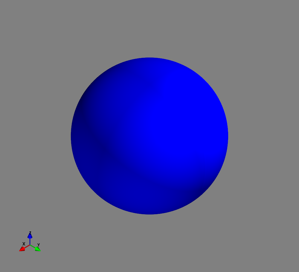
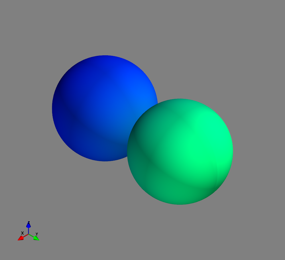
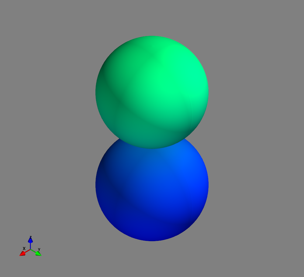
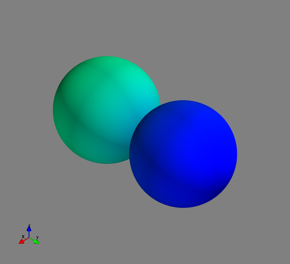
Fig.: Spherical harmonics :math:`Y_l^m left(vartheta, varphiright)` from left to the right: :math:`Y_{0}^{0}`, :math:`Y_{1}^{-1}`, :math:`Y_{1}^{0}`, and :math:`Y_{1}^{1}`. Note the swaped colors of the dumbbells, if changing :math:`m = -1 rightarrow +1`.

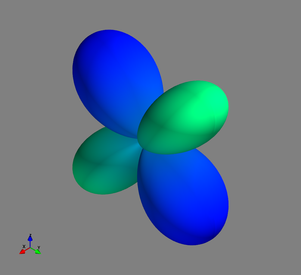
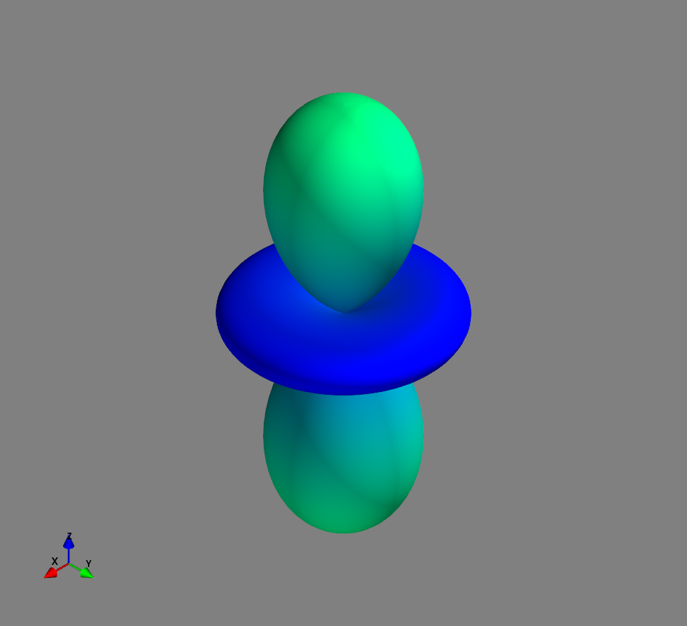
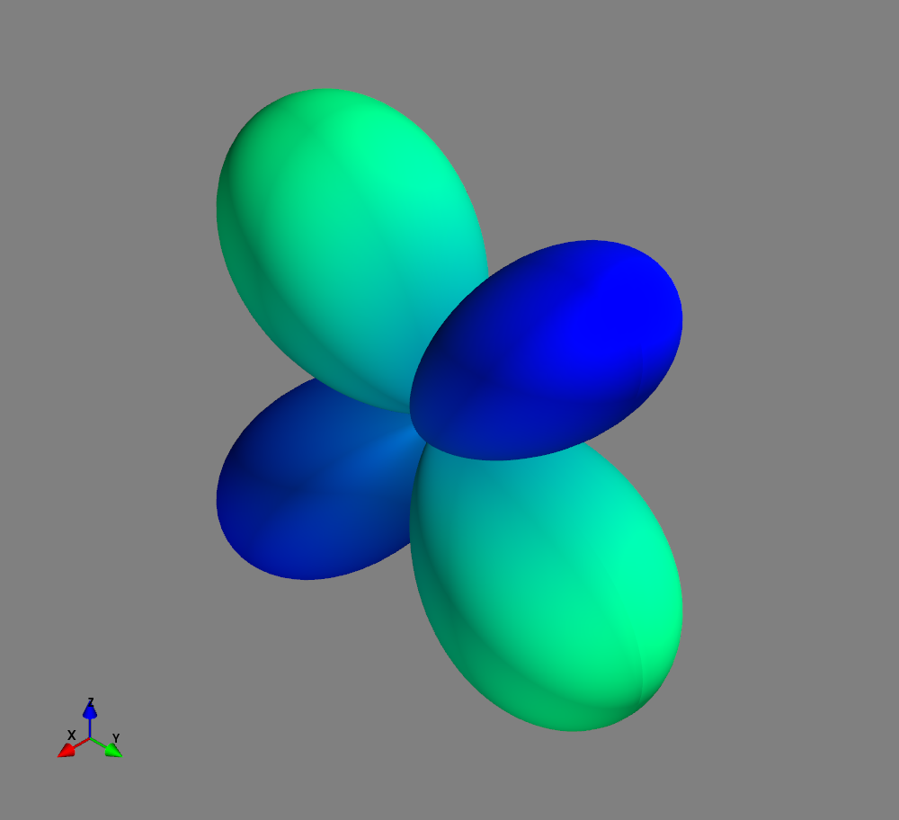
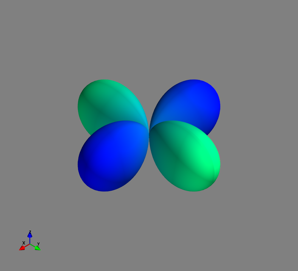
Fig.: Spherical harmonics :math:`Y_l^m left(vartheta, varphiright)` from left to the right: :math:`Y_{2}^{-2}`, :math:`Y_{2}^{-1}`, :math:`Y_{2}^{0}`, :math:`Y_{2}^{1}`, and :math:`Y_{2}^{2}`. Note the swaped colors of the dumbbells, if changing :math:`m = -1 rightarrow +1`. Changing :math:`m = -2 rightarrow +2` only affects the complex exponential function and is not visualized.

Solving the solution function $R\left(r\right)$

Previously we have derived the sperical harmonics and their squares as angular dependence of the probability density of a perticle within a spericaly symmetric potential. Now, we would like to solve the last dependence, namely the solution for the radial function $R\left(r\right)$. Above we have derived the constant $C_2$ with

$$\begin{array}{r}\begin{array}{rcl}{C}_2& =& l(l+1)\\ & =& \frac{1}{R\left(r\right)}\frac{\mathrm{d}}{\mathrm{d}r}\left(r^2\frac{\mathrm{d}R\left(r\right)}{\mathrm{d}r}\right)+\frac{2m}{{\hslash }^2}(E-V\left(r\right))r^2\end{array}.\end{array}$$

If we multiply this equation with $R\left(r\right)$ and divide through $r^2$, we obtain

$$\begin{array}{rcl}\frac{l(l+1)}{r^2}R\left(r\right)& =& \frac{1}{r^2}\frac{\mathrm{d}}{\mathrm{d}r}\left(r^2\frac{\mathrm{d}R\left(r\right)}{\mathrm{d}r}\right)+\frac{2m}{{\hslash }^2}(E-V\left(r\right))R\left(r\right)\end{array},$$

where the qunatum number $l$ denotes the angular momentum $\left|\overrightarrow{L}\right|=\sqrt{l(l+1)}\cdot \hslash$ of our quantum particle. If we now make use of the Coulomb potential

$$V\left(r\right)=-\frac{Z{e}^2}{4\pi {\epsilon }_{0}r}$$

as an example for a sperically symmetric potential and replace the mass $m$ by the reduced mass $\mu$ of an electron in the Coulomb potential of a nucleus with charge $Z\cdot e$ and mass $m_n\gg m_e$, as well as calculate the derivative of the first term, we obtain

$$\begin{array}{rcl}0& =& \frac{{\mathrm{d}}^{2}R\left(r\right)}{\mathrm{d}{r}^2}+\frac{2}{r}\frac{\mathrm{d}R\left(r\right)}{\mathrm{d}r}+(\frac{2\mu }{{\hslash }^2}(E+\frac{Z{e}^2}{4\pi {\epsilon }_{0}r})-\frac{l(l+1)}{r^2})R\left(r\right)\end{array}.$$

In order to solve this equation for $E<0$, we use the ansatz

$$R\left(r\right)=u\left(r\right)\cdot {\mathrm{e}}^{-\kappa r},$$

were we made use of the abbreviation

$$\kappa =\frac{\sqrt{-2E}}{\hslash }.$$

With the substtution

$$a=\frac{\mu Z{e}^2}{4\pi {\epsilon }_0{\hslash }^2}$$

we obtain

$$\begin{array}{rcl}0& =& \frac{{\mathrm{d}}^{2}u\left(r\right)}{\mathrm{d}{r}^2}+2(\frac{1}{r}-\kappa )\frac{\mathrm{d}u\left(r\right)}{\mathrm{d}r}+(2\frac{a-\kappa }{r}-\frac{l(l+1)}{r^2})u\left(r\right)\end{array}.$$

In order to solve this problem we use the ansatz of a power series

$$u\left(r\right)=\sum _j{b}_j{r}^j.$$

If we use this series in the differential equation and compare the coefficients, we obtain the recursive formula

$$b_j=2b_{j-1}\cdot \frac{\kappa \cdot j-a}{j(j+1)-l(l+1)}.$$

In order to normalize $R\left(r\right)$, the series has to have a finite number of elements. Furthermore, from the denomonator we get the condition $j<l$. Let us assume the element $j=n-1$ is the last non-zero element ($b_{n-1}\ne 0$) of this series, but the element $j=n$ ist the first element that is zero ($b_n=0$). Thus, we introduced the condition

$$j<n.$$

Furthermore, on the basis of the recursive formula we obtain

$$a=n\cdot \kappa$$

which leads to

$$\begin{array}{r}\begin{array}{rcl}E=-\frac{a^2{Z}^2}{2\mu n^2}& =& -\frac{\mu e^4}{8{\epsilon }_0^2{\hslash }^2}\frac{Z^2}{n^2}\\ & =& -R{y}^{\ast }\frac{Z^2}{n^2}=E_n.\end{array}\end{array}$$

The qunatization of the energy eigenstates arise from the condition $\psi (r⟶\mathrm{\infty })⟶0$. Furthermore, from the denominator of the recursive formula we derive

$$l\le j\le n-1$$

which leads to the condition for the quantum number of the angular momentum

$$l\le n-1.$$

On teh basis of teh recursicve formula w can calculate the function $u\left(r\right)$ and thus $R\left(r\right)$. This function $R\left(r\right)=R_{n,l}\left(r\right)$ depends on the principal quantum number $n$ (due to $j<n$ in the sum formula) and on the quantum number of the angular momentum $l$ (due to the recursive formula).

The first three normalized radial functions $R_{n,l}\left(r\right)$ are listed in the following table ($N={\left(Z/\left(a_{0}n\right)\right)}^{3/2}$, $x=Zr/\left(a_{0}n\right)$, $a_0=4\pi {\epsilon }_0{\hslash }^2/\left(\mu e^2\right)$).

$n$	$l$	$R_{n,l}\left(r\right)$
1	0	$2N{\mathrm{e}}^{-x}$
2	0	$2N{\mathrm{e}}^{-x}(1-x)$
2	1	$\frac{1}{\sqrt{3}}2N{\mathrm{e}}^{-x}x$
3	0	$2N{\mathrm{e}}^{-x}(1-2x+\frac{2}{3}{x}^2)$
3	1	$\frac{\sqrt{2}}{3}2N{\mathrm{e}}^{-x}x(2-x)$
3	2	$\frac{\sqrt{2}}{3\sqrt{10}}2N{\mathrm{e}}^{-x}{x}^2$

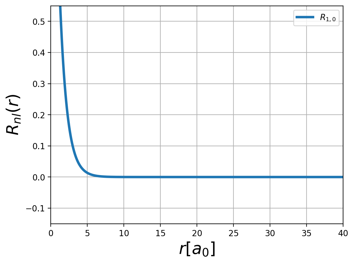
Fig.: (left) The radial function :math:`R_{n,l} left(rright)` and (right) the corresponding probability density :math:`left| R_{n,l} left(rright) right|^2` for :math:`n=1`.

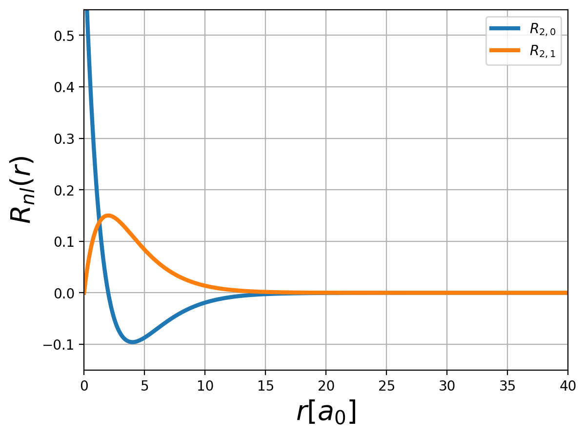
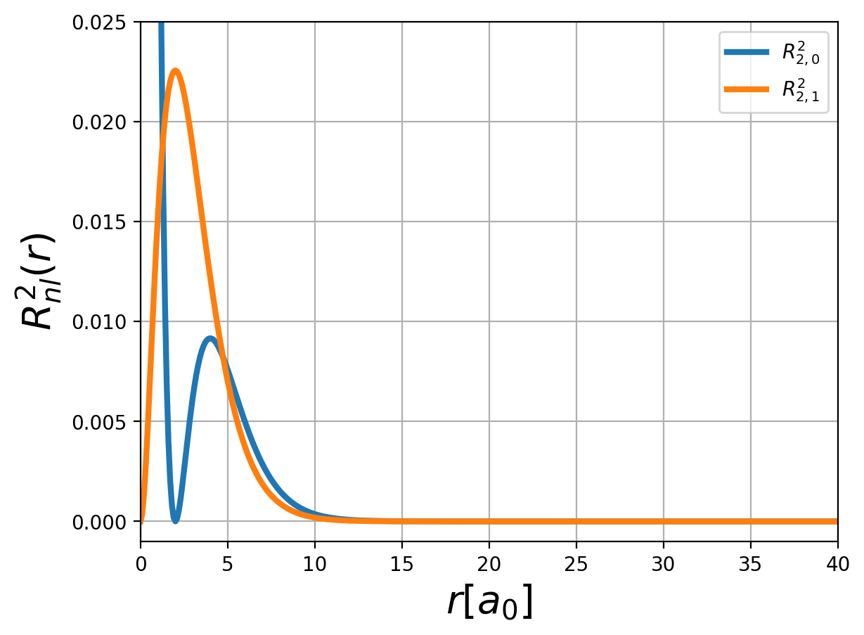
Fig.: (left) The radial function :math:`R_{n,l} left(rright)` and (right) the corresponding probability density :math:`left| R_{n,l} left(rright) right|^2` for :math:`n=2`.

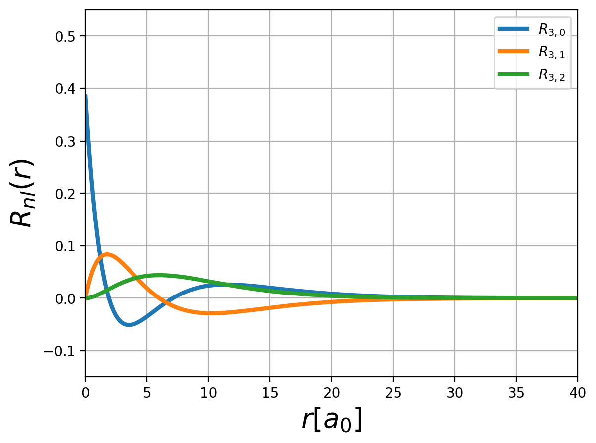
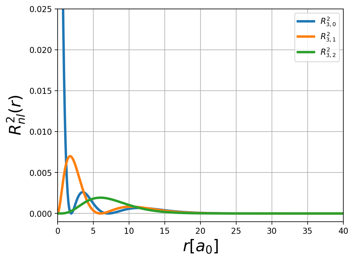
Fig.: (left) The radial function :math:`R_{n,l} left(rright)` and (right) the corresponding probability density :math:`left| R_{n,l} left(rright) right|^2` for :math:`n=3`.

We can see that the energy of a quantum state depends only on the principal quantum number $n$, but not on the other quantum numbers $l$ and $m$. Because $-l\le m\le +l$, there exists $2l+1$ energeticall equal (degenerated) states for every particular value of $l$. Furthermore, for every particular values of $n$, there exists

$$\sum _{l=0}^{n-1}(2l+1)=n^2$$

distinct states $(n,l,m)$ with $n^2$ distinct wave functions

$${\psi }_{n,l,m}(r,\vartheta ,\phi )=R_{n,l}\left(r\right)\cdot Y_l^m(\vartheta ,\phi )$$

.