This page was generated from `/home/lectures/exp3/source/notebooks/L19_AMA/Dipole Radiation.ipynb`_.

Dipole Radiation

We would like to have a look at the origin of electromagnetic radiation in a classical picture. Especially we would like to understand, why the electromagnetic fields that are radiated are transverse to the direction of propagation. We will consider for this purpose the radiation generated by an accelerated charge.

Electric field of an accelerated charge

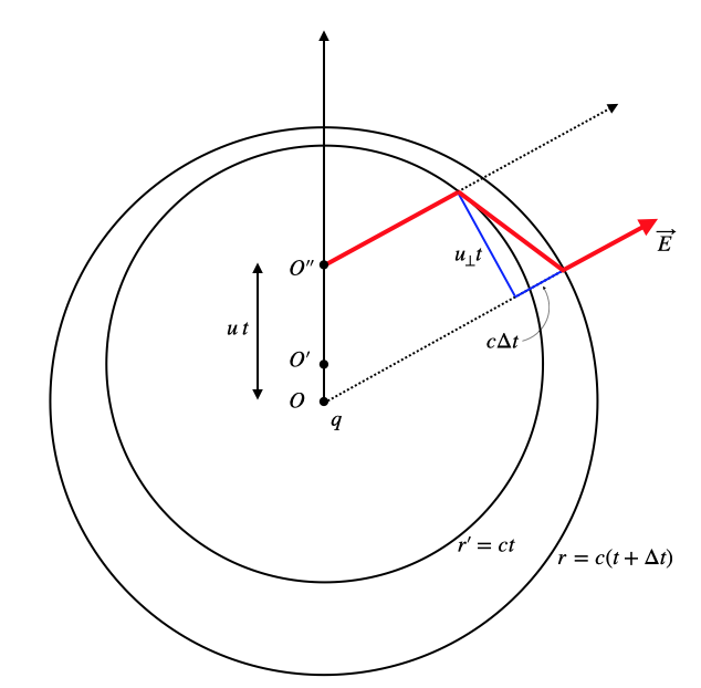
We will follow for the derivation of transverse electric field the basic steps of the derivation by Larmor. We consider a charge, which is initially at rest in the point \(O\) as sketched below. The charge is then accelerated for a very short period \(\Delta t\) to the point \(O'\) and reaches a final speed \(u\), which is small as compared to the speed of light \(u<<c\). The charge then moves with that speed up to a point \(O''\) for a time \(t\).

Fig.:

What will be important for our consideration is the fact that any information about a systems change of state is limited in its propagation to the speed of light. Thus, the information that the charge \(q\) has been accelerated has propagated from \(O\) a distance \(r=c(t+\Delta t)\), when the charge has reached the point \(O''\). The fact that the charge stopped accelerating, which is originating from point \(O'\) has traveled a distance \(r'=ct\).

Consider now the field line of the electric field that exists outside the outer circle which would trace back to point \(O\). This field line has now moved with the charge and is inside the inner circle corresponding to the red line. This field line needs to be connected to the remaining part outside the outer circle, as it is the same field line. Thus, the field line needs to bend accordingly in the shell between the circles as indicated by the red line.

The bend part of the field vector can be decomposed into a field component perpendicular (\(E_\perp\)) to the direction from \(O\) and one parallel to this radial direction (\(E_{||}\)). The perpendicular component is the new thing and we would like to calculate it.

The ratio of perpendicular and parallel component is then given by

\[\frac{E_{\perp}}{E_{||}}=\frac{u_{\perp}t}{c\Delta t}=\frac{a_{\perp}\Delta t t }{c\Delta t}\]

where the ratio of the electric fields is the same as of the velocity components. The velocity \(u_{\perp}\) thereby follows directly from the component of the acceleration perpendicular to the radial direction \(a_{\perp}\). The result of this calculation is then independent of the time period \(\Delta t\) and we obtain

\[E_{\perp}=\frac{a_{\perp}r}{c^2}E_{||}\]

where we replaced the time \(t\) by \(t=r/c\). To obtain \(E_{\perp}\) we now need to know the value of \(E_{\parallel}\), which we can obtain by Gauss theorem considering the a “pillbox” around the boundary of the sphere emanating from \(O\). Since the field lines from \(O\) are radially outwards, this calculation yields

\[E_{\perp}=-\frac{a_{\perp}}{c^2}\frac{q}{4\pi \epsilon_0 r^2}=-\frac{a_{\perp} q}{c^24\pi \epsilon_0 r}\]

This electric field that is generated is now not anymore radially pointing outwards from the source, but it is tangential to a sphere around \(O\). It further decays with the distance as \(1/r\) and not \(1/r^2\) as the common Coulomb field. The distance dependence is consistent with the one developed earlier for spherical waves. As we know that this electric field \(E_{\perp}\) is tangential to the sphere surface, we may write down the radiated field of the accelerated charge as

\[\vec{E}(\vec{r},t)=-\frac{a_{\perp}q}{c^2 4\pi \epsilon_0 r}\hat{\theta}\]

and the corresponding magnetic field as

\[\vec{B}(\vec{r},t)=\frac{\vec{E}}{c}=-\frac{a_{\perp}q}{c^3 4\pi \epsilon_0 r}\hat{\phi}\]

where \(\hat{\theta}\) and \(\hat{\phi}\) are the unit vectors along the polar and azimuthal direction.

Note that in the above equation the electric field is observed at time \(t\) but the acceleration has happened a time \(t-\frac{r}{c}\) earlier as it propagates with finite speed. This will finally lead our wavelike propagation.

Energy flow

With the help of the Poyting vector

\[\vec{S}(\vec{r},t)=\frac{1}{\mu_0} \vec{E} \times \vec{B}\]

we may now have a look at the energy flow from the accelerated charge. Since the electric and the magnetic field are orthogonal we can readily obtain the magnitude of the Poynting vector

\[S(\vec{r},t)=\frac{a_{\perp}^2 q^2}{\mu_0 c^5 (4\pi \epsilon_0)^2 r^2}\]

from which now follows with \(a_{\perp}=a\sin{\theta}\)

\[S(\vec{r},t)=\frac{a^2 q^2\sin^2(\theta)}{\mu_0 c^5 (4\pi \epsilon_0)^2 r^2}\]

or

\[S(\vec{r},t)=\frac{a^2 q^2\sin^2(\theta)}{c^3 (4\pi \epsilon_0)^2 r^2}\]

The total power that is then radiated by the accelerated charge is the given as the integral of the Poynting vector over a closed surface around the charge, i.e.

\[P=\int\int S dA=\frac{a^2 q^2\sin^2(\theta)}{c^3 (4\pi \epsilon_0)^2}\int_0^{2\pi}\int_{0}^{\pi}\frac{\sin^2(\theta)}{r^2}r^2 \sin(\theta) d\theta d\phi\]

which upon integration finally yields Larmor’s formula

\[P=\frac{q^2a^2}{6\pi c^3 \epsilon_0}\]

This is the total radiated power of an accelerated charge.

Oscillating Dipole

With the previous section we are now ready to have a look at a situation, where the charge is oscillating, for example, around a fixed positive charge. This situation can occur when an atom is polarized by teh electric field of an incident light wave. Since this electric field is in the visible range of a wavelength much longer than the size of the atom, we may consider the atom as being in a homogeneous oscillating electric field as we did already earlier. This approximation is called the Rayleight limit and the process is termed Rayleigh scattering. Let’s assume the charge is oscillating at a frequency \(\omega\) such that its displacement from the positive charge is

\[x=x_0 e^{i\omega t}\]

from which we obtain the velocity

\[\dot{x}=ix_0 \omega e^{i\omega t}\]

and finally the required acceleration

\[\ddot{x}=a=-x_0 \omega^{2}e^{i\omega t}\]

The product of charge and acceleration which enters the generated electric field can then be expressed as

\[q a=-q x_{0}\omega^{2}e^{i\omega t} = -p \omega^{2}e^{i\omega t}\]

since the dipole moment is given by \(p=q x_0\). Consequently, the electric field radiated by an oscillating dipole is given

\[E(\vec{r},t)=-\frac{a_{\perp} q}{c^24\pi \epsilon_0 r}=\frac{p\omega^2 \sin^2(\theta)}{c^2 4\pi\epsilon_0 r}e^{i\omega t}\]

The direction of the electric and also the magnetic field can now be constructed with the appropriate unit vector in the radial direction as well as the direction of the dipole moment \(\vec{p}\). The perpendicular component of the dipole moment including its direction is given by \((\hat{e}_r\times \vec{p})\times \hat{e}_r\) such that we obtain the electric and magnetic field in its vectorial beauty

\begin{eqnarray} \vec{E}(\vec{r},t) & = &\frac{\omega^2}{4\pi \epsilon_0 c^2 r}(\hat{e}_r\times \vec{p})\times \hat{e}_r e^{i(k r - \omega t)}\\ \vec{B}(\vec{r},t) & = &\frac{\omega^2}{4\pi \epsilon_0 c r}(\hat{e}_r\times \vec{p}) e^{i(k r - \omega t)} \tag{far field oscillating dipole} \end{eqnarray}

This corresponds to the radiated field of an oscillating dipole at large distances (\(r >>\lambda\)), which is called the far field. In the near field, there are additional components of the electric field which are not propagating and quickly decaying. The total electric field of an oscillating dipole is given by

\[\vec{E}(\vec{r},t)=\frac{\omega^3}{4\pi \epsilon_0 c^3} \left [ ((\hat{e}_r\times \vec{p})\times \hat{e}_r)\frac{1}{k r}+3(\hat{e}_r(\hat{e}_r\cdot \vec{p})-\vec{p})\left(\frac{1}{(k r)^3}-\frac{i}{(kr)^2} \right)\right] e^{i(kr -i \omega t)}\]

With the help of the dipole field we thus obtain the intensity radiated by an oscillating dipole at

\[I(\theta)=\frac{\omega^4|\vec{p}|^2}{32\pi^2 \epsilon_0 c^3}(1-\cos^2(\theta))\]

and the radiated power is given by

\[P=\frac{\omega^4 |\vec{p}|^2}{12\pi \epsilon_0 c^3}=\left (\frac{2\pi}{\lambda}\right )^4\frac{c|\vec{p}|^2}{12\pi \epsilon_0} \tag{radiated power of an oscillating dipole}\]

As frequencies not go as easily in our daily color language, we have converted that expression to contain the wavelength of light, which tells us, that the power radiated scales with the inverse of the wavelength to the power of four. This means for the visible light, that blue light is scattered much stronger than red light.