This page was generated from `/home/lectures/exp3/source/notebooks/L27_AMA/L27_potential_well.ipynb`_.

A potential well

… with infinite high walls

Now we want to discuss the case that a particle is only allowed to be located within a defined space. This case can be constructed by means of a potential well like

\[\begin{split}E_{\mathrm{pot}} \left( x \right) = \begin{cases} +\infty & \text{, if $x < 0$}\\ 0 & \text{, if $0 \le x \le a$}\\ +\infty & \text{, if $a < x$}\\ \end{cases} \mathrm{.}\end{split}\]

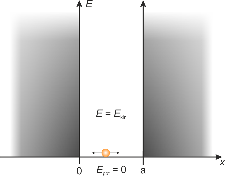
Fig.: A particle within a potential well with infinitely high walls.

Because the potential energy outside the potential well is infinite, it follows for the decay length \(\alpha = \sqrt{2 m \left( E_0 - E \right)}\),

\[\lim_{E_0 \to \infty} \alpha \left(E, E_0 \right) = \infty\]

and for the decay of the matter wave

\[\lim_{\alpha \to \infty} \mathrm{e}^{- \alpha x} = 0 \mathrm{.}\]

Thus, the penetration depth of the matter wave vanishes and we have “a particle in a box”. Within the region \(0 \le x \le a\) the potential energy is defined as \(0\), which is why we can state the stationary Schrödinger equation as discussed in the previous cases of a potential barrier,

\[\frac{\partial^2}{\partial x^2} \psi \left( x \right) + k^2 \psi \left( x \right) = 0 \mathrm{,}\]

and the solution for the position-dependent amplitude \(\psi \left( x \right)\) of the stationary Schrödinger equation,

\[\psi \left( x \right) = A \cdot \mathrm{e}^{+i k x} + B \cdot \mathrm{e}^{-i k x} \mathrm{.}\]

Because the potential energy outside the box approaches \(\infty\) and thus the propability density of our matter wave within these regions approaches \(0\), we state the boundary conditions

\[\begin{split}\begin{eqnarray} \psi \left( x \le 0 \right) & = & 0\\ \psi \left( x \ge a \right)& = & 0 \end{eqnarray}\end{split}\]

and obtain

\[\begin{split}\begin{eqnarray} A + B & = & 0\\ A \cdot \mathrm{e}^{+i k a} + B \cdot \mathrm{e}^{-i k a} & = & 0\mathrm{.} \end{eqnarray}\end{split}\]

On the basis of the first condition (\(B = -A\)) we refine the wavefunction

\[\psi \left( x \right) = A \left( \mathrm{e}^{+i k x} - \cdot \mathrm{e}^{-i k x} \right) = 2 i A \sin \left( k x \right)\]

and on the basis of the second condition (\(2 i A \sin \left( k a \right) = 0\)) we obtain

\[k \cdot a = n \cdot \pi \mathrm{.}\]

We refine the wave function further resulting in

\[\psi \left( x \right) = C \sin \left(n \frac{\pi}{a} x \right)\]

with \(C = 2 i A\). The last equation represents the maximum amplitude of a standing wave with the allowed wavenumbers and wavelengths being

\[\begin{split}\begin{eqnarray} k_{\mathrm{n}} & = & n \frac{\pi}{a}\\ \lambda_{\mathrm{n}} & = & \frac{2 a }{n} \mathrm{,} \end{eqnarray}\end{split}\]

respectively.

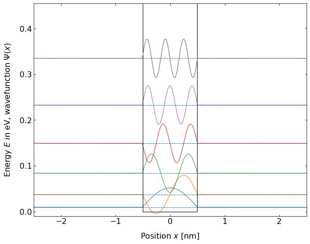
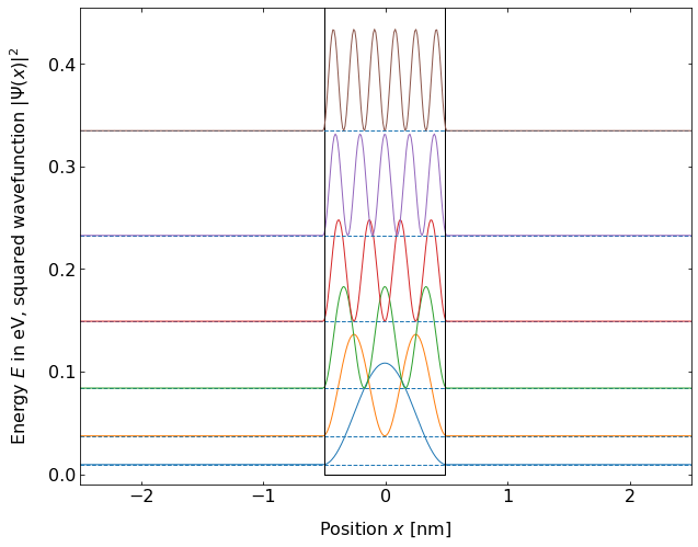
Fig.: (left) Wave functions :math:`psi_{mathrm{n}}` positioned at the height corresponding to the energy eigenvalue :math:`E_{mathrm{n}}`. (right) The according probability densities (squared wave functions). The postential is :math:`0` for :math:`-0.5 , mathrm{nm} le x le 0.5, mathrm{nm}`, otherwise it is set :math:`10^4 ; mathrm{eV}`

As the values that the wavenumber and wavelength can adopt are restricted in accorded to the boundary conditions, we are wondering how the energy of the particle might be affect. For the energy we can write

\[E = \frac{p^2}{2m} = \frac{\hbar^2 k^2}{2m} = \frac{\hbar^2}{2m} \left(\frac{n \pi}{a} \right)^2 = E_{\mathrm{n}}\]

and we see that our particle in the box cannot adopt any arbitray energy. In order to remain at a stationary state the particle can adopt only specific, descrete values of energy. Thus, the energy eigenvalues or energy principal values are quantized. We can state the energy \(E_{\mathrm{n}}\) in dependence of \(n\) as

\[E_{\mathrm{n}} = E_{\mathrm{1}} \cdot n^2 = \frac{\hbar^2}{2m} \frac{\pi^2}{a^2} \cdot n^2\mathrm{.}\]

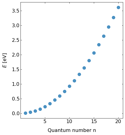
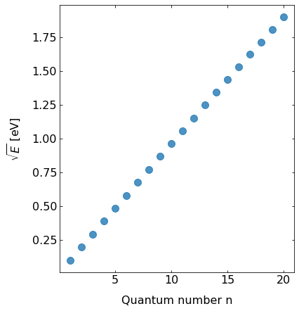
Fig.: (left) The energy eigenvalus in dependence of the quantum number :math:`n`. (right) The square root of the energy eigenvalues from the left panel in dependence of teh quantum number form a straight line, because of the :math:`E_n = E_1 cdot n^2` relation. The postential is :math:`0` for :math:`-0.5 le x le 0.5`, otherwise it is set :math:`10^4`

It is evident that the energy eigenvalues rise with the square of the quantum number (\(E_{\mathrm{n}} \propto n^2\)) and with the square of the inverse width of our potential well (\(E_{\mathrm{n}} \propto 1/a^2\)). Furthermore, the minimum energy \(E_{\mathrm{1}}\) is non-zero, its is rather

\[E_{\mathrm{1}} = \frac{\hbar^2}{2m} \frac{\pi^2}{a^2} > 0 \mathrm{.}\]

Only for an infinitely wide potential well \(E_{\mathrm{1}}\) approaches \(0\). The non-zero minimum energy is a consequence of Heisenbger’s uncertanty relation. If we restrict the particle in its position like \(\Delta x = a\), it follows for the momentum \(p \ge \Delta p \ge h/2\) which leads to \(k_{\mathrm{min}} = p_{\mathrm{min}}/\hbar = \pi/a\) and \(\lambda_{\mathrm{max}} = 2a\). If we use \(p_{\mathrm{min}}\) and calculate the minimum energy like \(E_{\mathrm{min}} = p^2_{\mathrm{min}} / \left( 2m \right)\) we obtain \(E_{\mathrm{min}} = E_{\mathrm{1}}\).

… with finite high walls

If the walls of the potential well are not of infinit height, the wave function might penetrate into the walls (\(x<0\) and \(x>a\)) and decay there exponentially (\(\propto \mathrm{e}^{-\alpha x}\)). Compared to the case with infinite high walls the wave functions are altered, because the boundary conditions in the previous form \(\psi \left( x \le 0 \right) = 0\) and \(\psi \left( x \ge a \right) = 0\) are no longer valied. The less the relative energy \(\left( E_{\mathrm{n}} - E_0\right)/E_0\) the more pronounced the deviation from the case of infinitely high walls (or an infinitely deep potential well).

Because the wavefunction is able to intrude into the walls, the position uncertainty \(\Delta x\) is increased. Thus, the momentum uncertainty is decreased compared to the previous case and the energy eigenvalues \(E_{\mathrm{n}}\) are reduced.

In oder to resolve the eigenstates, we state the general solution for the wave function in the regions as follows:

\[\begin{split}\psi \left( x \right) = \begin{cases} \psi_{\mathrm{-1}} \left( x \right) & \text{, if $x < 0$}\\ \psi_{\mathrm{0}} \left( x \right) & \text{, if $0 \le x \le a$}\\ \psi_{\mathrm{+1}} \left( x \right) & \text{, if $a < x$} \end{cases}\end{split}\]

with

\[\begin{split}\begin{eqnarray} \psi_{-1} & = & A_{-1} \mathrm{e}^{+ \alpha x} + B_{-1} \mathrm{e}^{- \alpha x}\\ \psi_{0} & = & A_{0} \mathrm{e}^{+ i k x} + B_{0} \mathrm{e}^{-i k x}\\ \psi_{+1} & = & A_{+1} \mathrm{e}^{+ \alpha x} + B_{+1} \mathrm{e}^{- \alpha x} \end{eqnarray}\end{split}\]

with \(\alpha = \sqrt{2m\left( E_0-E \right)}/\hbar\). Since the wave function has to be normalizable (in order to bear a reasonable physical meaning), we have to set \(B_{-1} = 0\) as well as \(A_{+1} = 0\). Furthermore, we redefine \(\psi_0\) resulting in

\[\psi_{0} = A_{0}^{\prime} \cos \left( k x \right) + B_{0}^{\prime} \sin \left( k x \right) \mathrm{,}\]

where \(A_{0}^{\prime} = A_0 + B_0\) and \(B_{0}^{\prime} = i \left( A_0 - B_0 \right)\).

If we now apply the boundary conditions at \(x = 0\), namely

\[\begin{split}\begin{eqnarray} \psi_{-1} \left( x = 0 \right) & = & \psi_{0} \left( x = 0 \right) \; \; \mathrm{and}\\ \frac{\partial}{\partial x} \psi_{-1} \left( x = 0 \right) & = & \frac{\partial}{\partial x} \psi_{0} \left( x = 0 \right) \end{eqnarray}\end{split}\]

we get

\[\begin{split}\begin{eqnarray} A_{-1} & = & A_0^{\prime} \; \; \mathrm{and}\\ \alpha A_{-1} & = & k B_0^{\prime} \end{eqnarray}\end{split}\]

respectively. From the boundary conditions at \(x = a\), namely

\[\begin{split}\begin{eqnarray} \psi_{0} \left( x = a \right) & = & \psi_{+1} \left( x = a \right) \; \; \mathrm{and}\\ \frac{\partial}{\partial x} \psi_{0} \left( x = a \right) & = & \frac{\partial}{\partial x} \psi_{+1} \left( x = a \right) \end{eqnarray}\end{split}\]

we get

\[\begin{split}\begin{eqnarray} A_{0}^{\prime} \cos \left( k a \right) + B_{0}^{\prime} \sin \left( k a \right) & = & B_{+1} \mathrm{e}^{- \alpha a} \; \; \mathrm{and}\\ -A_{0}^{\prime} k \sin \left( k a \right) + B_{0}^{\prime} k \cos \left( k a \right) & = & -\alpha B_{+1} \mathrm{e}^{- \alpha a} \mathrm{.} \end{eqnarray}\end{split}\]

If we divide the last equation by the second last and make use of \(B_{0}^{\prime} / A_{0}^{\prime} = \alpha / k\) from the boundary \(x = 0\), we derive the transient equation

\[2 \alpha k = \left( k^2 - \alpha^2 \right) \, \tan \left(k a \right)\]

which has the two solutions for \(\alpha\)

\[\begin{split}\begin{eqnarray} \alpha_{+} & = & k \cdot \tan \left( \frac{ak}{2} \right)\\ \alpha_{-} & = & -k \cdot \cot \left( \frac{ak}{2} \right) \mathrm{.} \end{eqnarray}\end{split}\]

On the basis of this solutions and the relations \(\alpha = \sqrt{ 2 m \left(E_0 -E \right)} /\hbar\) and \(k = \sqrt{2 m E} /\hbar\) we can calculate conditions for the energy eigenvalues \(E_{\mathrm{+}}\) and \(E_{\mathrm{-}}\) and the solutions for \(\alpha_{+}\) and \(\alpha{-}\) as follows

\[\begin{split}\begin{eqnarray} \tan \left( \frac{a}{2\hbar} \sqrt{2 m E_{+}} \right) & = & \sqrt{ \frac{E_0}{E_{+}}-1}\\ - \cot \left( \frac{a}{2\hbar} \sqrt{2 m E_{+}} \right) & = & \sqrt{ \frac{E_0}{E_{-}}-1}\mathrm{.} \end{eqnarray}\end{split}\]

These solutions for the energy eigenvalues \(E_{+/-}\) correspond to the symmetric and antisymmetric wavefunctions

\[\begin{split}\begin{eqnarray} \psi \left( x \right) & = & \psi_{+} \left( x \right) + \psi_{-} \left( x \right) \\ {} & = & A_0^{\prime} \cos \left( k x \right) + B_0^{\prime} \sin \left( k x \right) \mathrm{.} \end{eqnarray}\end{split}\]

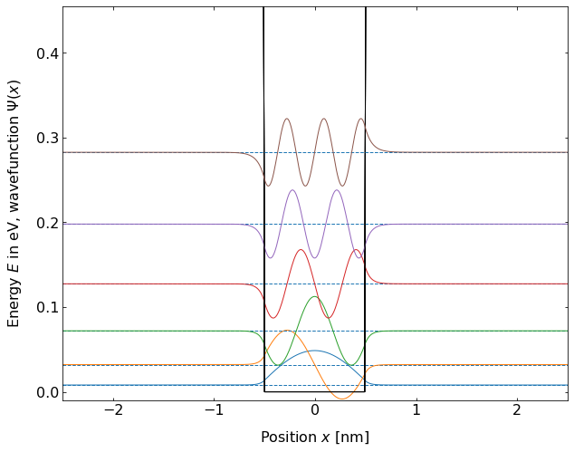
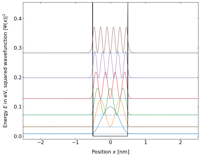
Fig.: (left) Wave functions :math:`psi_{mathrm{n}}` positioned at the height corresponding to the energy eigenvalue :math:`E_{mathrm{n}}`. (right) The according probability densities (squared wave functions). The postential is :math:`0` for :math:`-0.5 , mathrm{nm} le x le 0.5, mathrm{nm}`, otherwise it is set to :math:`0.5 ; mathrm{eV}`

In the case of an infinite deep potential well (\(E_0 \longrightarrow \infty\)} the tangens and cotanges functions approach \(\infty\). Then, we obtain the identical conditions for standing waves as dicussed on the above example of “a particle in a box”.

If the energy of the particle is greater than the depth of the potential well (\(E > E_0\)), then the energy eigenstates are no longer quantized. In contrast to the discrete states within the well, the particle is now in the so-called continuum and might adopt any arbitrary energy value. However, a matter with sufficient energy (\(E>E_0\)) will not pass the potential well without being influenced. As previously discussed on the examples of the different potential barriers, the wave will be in part reflected at the positions of the walls, even though the energy of the wave is much higher than the potetial well’s depth.

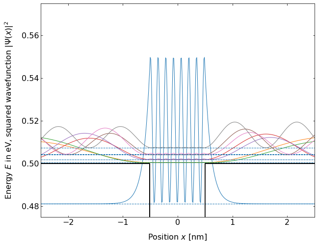
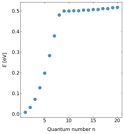
Fig.: (left) The probability densities :math:`left| psi_{mathrm{n}} right|^2` positioned at the height corresponding to the energy eigenvalue :math:`E_{mathrm{n}}` in the case of teh last bound state (:math:`n = 8`) and the next seven states. (right) The energy eigenvalues in dependence of teh quantum number. The postential is :math:`0` for :math:`-0.5 , mathrm{nm} le x le 0.5, mathrm{nm}`, otherwise it is set to :math:`0.5 ; mathrm{eV}`- Please not that the representation of the continuous states is only ofexemplary nature. The data are the actual results from the very same calculations as for the bound states. However, the description of the continuum might suffer from numerical resolution and calculation accuracy.