This page was generated from `/home/lectures/exp3/source/notebooks/L14/Reflection and Refraction.ipynb`_.

Reflection and Refraction of Electromagnetic Waves

Before we have a look at the behavior of electromagnetic waves at boundaries, we would like to setup the stage for those consideraations. For this purpose we need to define the geometry we are referring to and also have a look at the electric fields (and magnetic fields) that will be present. The sketch below shows the wavevectors of the incident ${\overrightarrow{k}}_I$, reflected ${\overrightarrow{k}}_R$ and transmitted ${\overrightarrow{k}}_T$ waves in the two materials with the refractive indices $n_1$ and $n_2$.

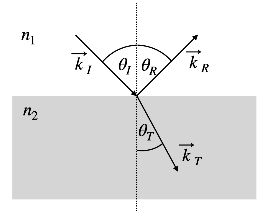
Fig.: Polarization of an electric cloud of an atom.

These wavevectors are connected to the following plane waves, we will consider. We will first assume that these three waves have different frequencies as well, even though we may guess that they have the same as they all stem from the incident wave.

$$\begin{array}{}\text{(incident)}& {\overrightarrow{E}}_{\mathrm{i}\mathrm{n}\mathrm{c}}={\overrightarrow{E}}_I{e}^{i({\omega }_{I}t-{\overrightarrow{k}}_I\cdot \overrightarrow{r})}\end{array}$$

$$\begin{array}{}\text{(reflected)}& {\overrightarrow{E}}_{\mathrm{r}\mathrm{e}\mathrm{f}}={\overrightarrow{E}}_R{e}^{i({\omega }_{R}t-{\overrightarrow{k}}_R\cdot \overrightarrow{r})}\end{array}$$

$$\begin{array}{}\text{(transmitted)}& {\overrightarrow{E}}_{\mathrm{t}\mathrm{r}\mathrm{a}}={\overrightarrow{E}}_T{e}^{i({\omega }_{T}t-{\overrightarrow{k}}_T\cdot \overrightarrow{r})}\end{array}$$

What we have to consider, however, is the direction of polarization of their electric or magnetic fields. This is important and shall not be confused in the following. We will differentiate between

• p-polarized light: electric field is in the plane of incidence (given by the k-vector and the surface normal), also called transverse magnetic (TM)

• s-polarized light: electric field is perpendicular to the plane of incidence, also called transverse electric (TE)

This is sketched in the image below.

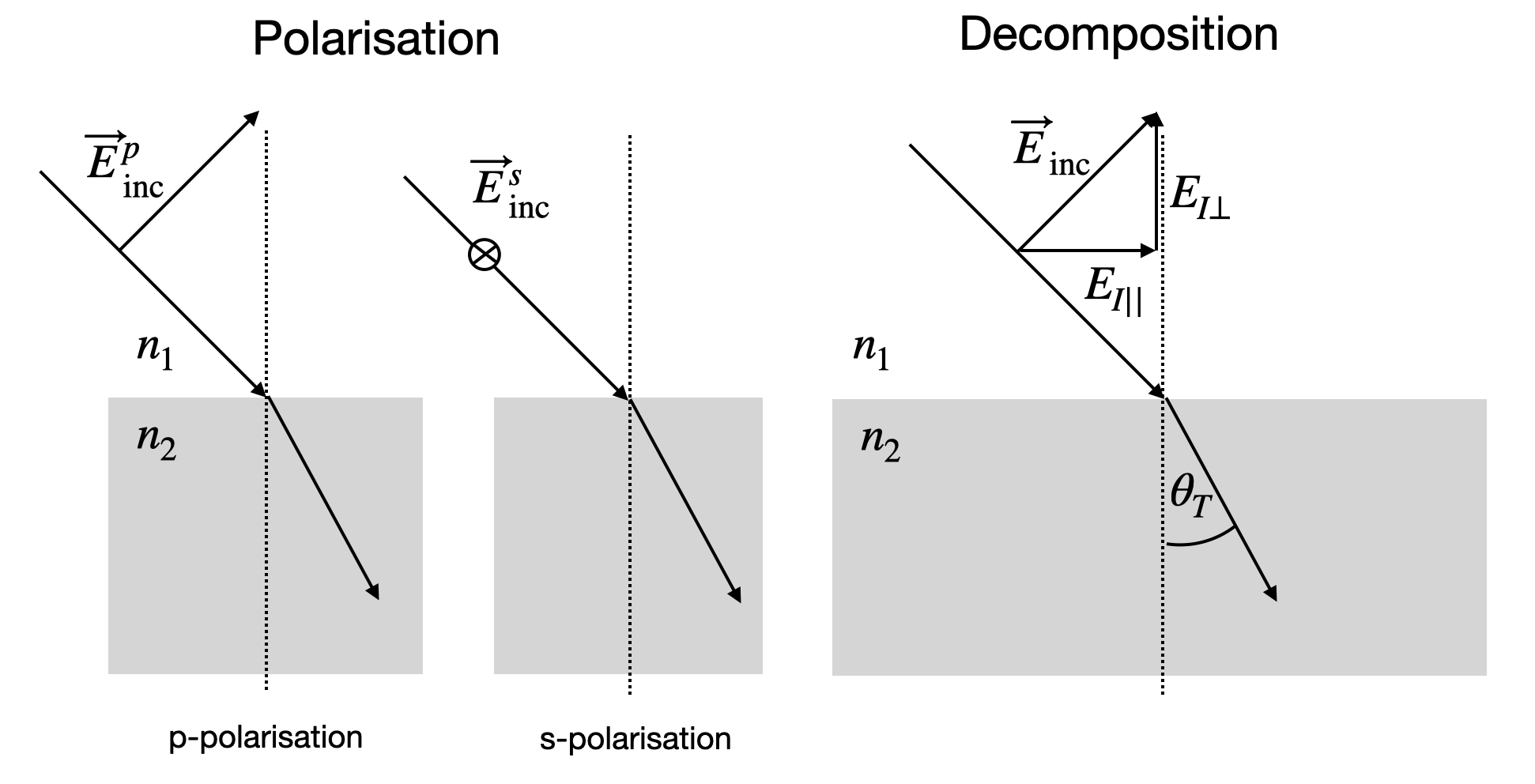
Fig.: Polarization of an electric cloud of an atom.

To apply the boundary conditions, we will further need to split thesse polarisation vectors into components, which are parallel ($||$) or perpendicular ($\perp$) to the interface. This is required as we will have boundary conditions for the electric and magnetic fields either parallel or perpendicular to the interface. The s-polarisation, for example, has an electric field, which is always parallel to the interface, while the p-polarization comprises both components.

Boundary Condition

The boundary conditions fo rthe electric or magnetic field passing an interface are derived from the Maxwell equations. As I assume you have don this already in the electro- and magnetostatics lectures, I will only resume shortly here.

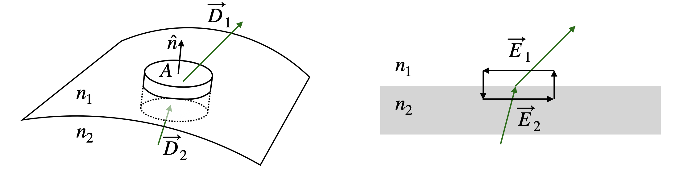
Fig.: Polarization of an electric cloud of an atom.

Let us take the divergence of the displacement field $\mathrm{\nabla }\cdot \overrightarrow{D}={\rho }_f$ which is equal to the density of free charges. When integrating both sides over the volume

$$\int \mathrm{\nabla }\overrightarrow{D}dV=\int {\rho }_{f}dV$$

we can apply Gauss’ theorem and replace the volume integral over the divergence with an integral over closed surface of that volume

$$\oint \overrightarrow{D}d\overrightarrow{A}=q_f$$

where $d\overrightarrow{A}$ is a vector standing perpendicular on the surface element $dA$ and $q_f$ are the free charges in the volume. If we now consider a volume, which has the shape of a pillbox as displayed in the above sketch on the left side, we may let the height of the volume contract to zero and write the surface integral as

$$({\overrightarrow{D}}_2-{\overrightarrow{D}}_1)\cdot \hat{n}=q_f/A={\sigma }_f$$

where $A$ is the cap area of the cylinder and $\hat{n}$ is a unit vector directed from material 2 to material 1. As the unit vector $\hat{n}$ is perpendicular to the interface, this states that the difference in the normal components of the displacement field is due to free surfaces charges. Thus in the case of no free charges at the interface (${\sigma }_f=0$), the normal components of the displacement field is conserved across the interface.

$$\begin{array}{}\text{(for }{\sigma }_f=0\text{)}& D_{1\perp }=D_{1\perp }\end{array}$$

This also says that there is a jump in the normal electric field component

$$\frac{E_{1\perp }}{E_{2\perp }}=\frac{{ϵ}_2}{{ϵ}_1}$$

as $D=ϵE$. A similar calculation can also be done with the magnetic flux density $\mathrm{\nabla }\cdot \overrightarrow{B}=0$, which yields tha the normal component of the flux density is conserved as well, but the magnetic field normal component has a jump according to the magnetic permeabilities ${\mu }_1,{\mu }_2$.

The right sketch in the above Figure indicates the calculations that yield the boundary conditions for the parallel components of the electric and magnetic field. Here we use the Maxwell equation

$$\mathrm{\nabla }\times \overrightarrow{E}=-\frac{\partial \overrightarrow{B}}{\partial t}$$

Integrating both sides over an area allows us to use Stokes theorem, stating that the integral over the rotation of an electric field can be transformed into a closed loop integral over the electric field.

$$\oint \overrightarrow{E}d\overrightarrow{l}=-\frac{\partial }{\partial t}\int \overrightarrow{B}d\overrightarrow{A}$$

Letting the area go to zero as well, we find

$$\hat{n}\times ({\overrightarrow{E}}_2-{\overrightarrow{E}}_1)=0$$

or

$$E_{2||}=E_{1||}$$

saying that the tangential component of the electric field is conserved. In the case of zero surface currentsm, this is also true for the magnetic field ($\overrightarrow{H}$) components along the interface.

Reflection/Refraction

We can now continue to calculate the mathcing of frequency and wavevector at the interface as well consider the amplitudes of the electric and magnetic fields.

Frequency and Wavevector Matching

Recalling the above formulas for the incident, reflected and transmitted plane waves, we can explicitely write down the components of the wavevectors of the three waves in our cordinate system

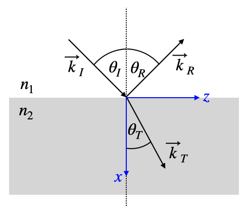
Fig.:

According to that drawing, we have

$$\begin{array}{rcl}{\overrightarrow{k}}_I& =& k_I\cos ({\theta }_I){\hat{e}}_x+k_I\sin ({\theta }_I){\hat{e}}_z\\ {\overrightarrow{k}}_R& =& -k_R\cos ({\theta }_R){\hat{e}}_x+k_R\sin ({\theta }_R){\hat{e}}_z\\ {\overrightarrow{k}}_T& =& k_T\cos ({\theta }_T){\hat{e}}_x+k_T\sin ({\theta }_T){\hat{e}}_z\end{array}$$

Note that the component ${\hat{e}}_x$ always provides the wavevector component perpendicular to the interface, while ${\hat{e}}_z$ is the tangential (parallel) component. The total field in both sides is given by

$$\begin{array}{}\text{(}x<0\text{)}& \overrightarrow{E}={\overrightarrow{E}}_{\mathrm{i}\mathrm{n}\mathrm{c}}+{\overrightarrow{E}}_{\mathrm{r}\mathrm{e}\mathrm{f}}\end{array}$$

and

$$\begin{array}{}\text{(}x>0\text{)}& \overrightarrow{E}={\overrightarrow{E}}_{\mathrm{t}\mathrm{r}\mathrm{a}}\end{array}$$

on the other side. We now want that those field mathc according to our previously described boundary conditions.

This matching of the field shall be valid at all times, which directly requires

$$\begin{array}{}\text{(frequency mathcing)}& {\omega }_I={\omega }_R={\omega }_T\end{array}$$

This is what we already guessed. Along the interface we also need to have a phase mathcing of the waves as already discussed in the wave optics chapter. This means that

$${\overrightarrow{k}}_I\cdot \overrightarrow{r}={\overrightarrow{k}}_R\cdot \overrightarrow{r}={\overrightarrow{k}}_T\cdot \overrightarrow{r}$$

at all positions $\overrightarrow{r}$ that belong to the interface (i.e. $x=0$). Therefore $\overrightarrow{r}=\{0,y,z\}$ and the equalities yield

$$k_I\sin ({\theta }_I)=k_R\sin ({\theta }_R)=k_T\sin ({\theta }_T)$$

Since the magnitude of the wavevector of the incidenet and the reflected light is the same (both wave travel in the same material), we immediately find

${\theta }_I={\theta }_R$

For the incident and the transmitted wave we have to take the change of the wavenumber into account, which gives.

$$\begin{array}{rcl}{n}_1{k}_0\sin ({\theta }_I)& =& n_2{k}_0\sin ({\theta }_T)\\ n_1\sin ({\theta }_I)& =& n_2\sin ({\theta }_T)\end{array}$$

which is Snells law. Snells law is the result of the conservation of the parallel component of the wavevector across an interface, while the normal component has to have a jump according to the refractive indices.