This page was generated from `/home/lectures/exp3/source/notebooks/L24_AMA/L24_Heisenbergs_uncertainty_relation.ipynb`_.

Heisenbergs Uncertainty Relation

Position-momentum uncertainty

As an example for a wave packet we chose plane waves whose amplituds obey a Gaussian distribution centered at \(k_0\),

\[C \left( k \right) = C_0 \, \mathrm{e}^{- \left( \frac{a}{2}\right)^2 \left( k - k_0\right)^2 } \mathrm{.}\]

Then the one-dimensional wave packet results in

\[\psi \left( z,t \right) = C_0 \int_{-\infty}^{+\infty} \mathrm{e}^{- \left( \frac{a}{2}\right)^2 \left( k - k_0\right)^2 } \, \mathrm{e}^{i\left(k z - \omega t\right) } \, \mathrm{d}k \mathrm{.}\]

We examine the integration and determine for the case of \(t=0\) the normalization constant \(C_0 = \sqrt{a} \, \left( \pi \right)^{3/4}\). The wave packet and propability denisty then read as

\[\psi \left( z,0 \right) = \left(\frac{2}{\pi a^2} \right)^{\frac{1}{4}} \cdot \mathrm{e}^{- \left( \frac{z}{a} \right)^2} \, \mathrm{e}^{i k_0 z}\]

and

\[\left| \psi \left( z,0 \right) \right|^2 = \sqrt{\frac{2}{\pi a^2} } \cdot \mathrm{e}^{- 2 \left( \frac{z}{a} \right)^2} \mathrm{,}\]

respectively. The latter obye the normalization condition.

Our wave packet exhibits a maximum at \(z=0\). At \(z_{1,2} = \pm a/2\) the propability density drops to \(\left| \psi \left( z,0 \right) \right|^2 = 1/\sqrt{\mathrm{e}}\) of teh maximum. Commonly, the width \(z_1 - z_2 = \Delta z = a\) is defined as full width of the wave packet.

Concerning the wave number, the wave packet is comprised of plane waves which obey the amplitude distribution \(C\left( k \right)\). If we know wonder for the width \(\Delta k = k_1 - k_0\) fulfilling the condition \(\left| C \left( k \right) \right|^2 = C_0^2/\sqrt{\mathrm{e}}\), it deriectly follows \(\Delta k = 1/a\).

Now we can conclude, the product of the spatial width of the wave packet \(\Delta z\) and the width of the wavenumber interval \(\Delta k\) equals \(1\),

\[\Delta z \cdot \Delta k = 1 \mathrm{.}\]

A first indication of this fact you got already when introducing wave packets. As depicted, the broader the wavenumber intervall, the narrower the width in z. The meaning of the condition between \(\Delta z\) and \(\Delta k\) becomes clear, if we use the momentum on the basis of the de Broglie wavelength \(p_z = \hbar k\). Then, the product reads as \(\Delta z \cdot \Delta p_z = \hbar\). In the case of a Gaussian distribution, the product \(\Delta z \cdot \Delta p_z = \hbar\) is the smallest. In the case of any other distribution function, the product is larger \(\Delta z \cdot \Delta p_z > \hbar\). On teh basis of these consideration, we can formulate Heisenberg’s uncertainty relation,

\[\Delta z \cdot \Delta p_z \ge \hbar \mathrm{.}\]

For the other two directions of the three-dimentional space one obtains analogously

\[\begin{split}\begin{eqnarray} \Delta x \cdot \Delta p_x & \ge & \hbar\\ \Delta y \cdot \Delta p_y & \ge & \hbar \end{eqnarray}\end{split}\]

Often the spatial width \(\Delta z\) is defined as the width where the wave packet drops to \(1/\mathrm{e}\) of the maximum amplitude. Then it follows for the spatial width \(\Delta z = \sqrt{2} \, a\) and for the wavenumber interval \(\Delta k = \sqrt{2}/a\). As a consequence the product \(\Delta z \cdot p_z = 2 \hbar\).

If we assume a constant amplitude (as we did for introducing matter waves inteh previous chapter), we might also define the distance between the first root at either side as width of the wave packet. The root is located at \(u_{\mathrm{root}} = 2 \pi / \Delta k\). Making use of \(u = \left(\mathrm{d}\omega / \mathrm{d} k \right)_{k_0} - z\) it follows \(\Delta z = 4 \pi / \Delta k\) and \(\Delta z \cdot \Delta k \ge 4 \pi\). As a consequence, the uncertainty relation reads as \(\Delta z \cdot \Delta p_z \ge 2 h\) with \(h = 2 \pi \hbar\).

Thus, the exact value of the limit of \(\Delta z \cdot \Delta p_z\) does depent on the definition of the spatial uncertainty \(\Delta z\) and in accord \(\Delta p_z\).

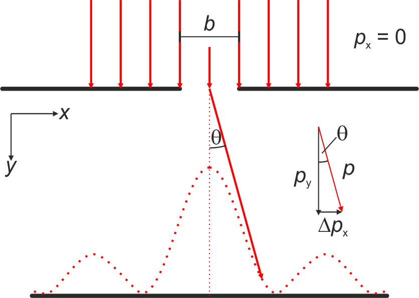
One illustrative example is provided on the basis on electron diffraction at a single slit. Let us assume a single slit parallel to the \(x\) axis with a width of \(\Delta x = b\) and an electron beam with the momentum \(\vec{p} = \left( 0,p_y,0 \right)^{\mathrm{T}}\). Before the electrons pass the slit their momentum along \(x\) is \(p_x = 0\), while we cannot provide any details about their \(x\) coordinate. At the slit only those electrons can pass whose \(x\) coordinate is in the interval between \(x = 0 - b/2\) and \(x = 0 + b/2\). Thus, for the transmitted electron we can constrain the space of possible \(x\) values down to \(\Delta x = b\) and in accord to the uncertainty relation the momentum along the \(x\) direction becomes \(p_x \ge \hbar / b\). As a consequence, after passing the slit the electrons are distributed about an angle \(-\theta \le \varphi \le + \theta\) with the condition

\[\sin \left( \theta \right)= \frac{\Delta p_x}{p} = \frac{h}{bp} \mathrm{.}\]

If we describe the electrons by means of the de Broglie wavelength \(\lambda = p/h\), then the wave is diffracted at the slit and we get a central maximum of the diffraction pattern with the width \(\Delta \varphi = 2 \theta\). Analogously to the diffraction of light we get

\[\sin \left( \theta \right)= \frac{\lambda}{b} \mathrm{.}\]

On the basis of this exmaple we see that the uncertainty arise from the description of a particle as wave and the spatial constraints of this wave.

Fig.: Scheme of an electron with a momentum uncertainty along :math:`x` of :math:`Delta p_x = 0` and thus :math:`Delta x = infty` before it enters the slit. Due to the localization through the slit (:math:`Delta x` becomes a finite number), the electron experiences an uncertainty of the momentum :math:`Delta p_x > 0`.

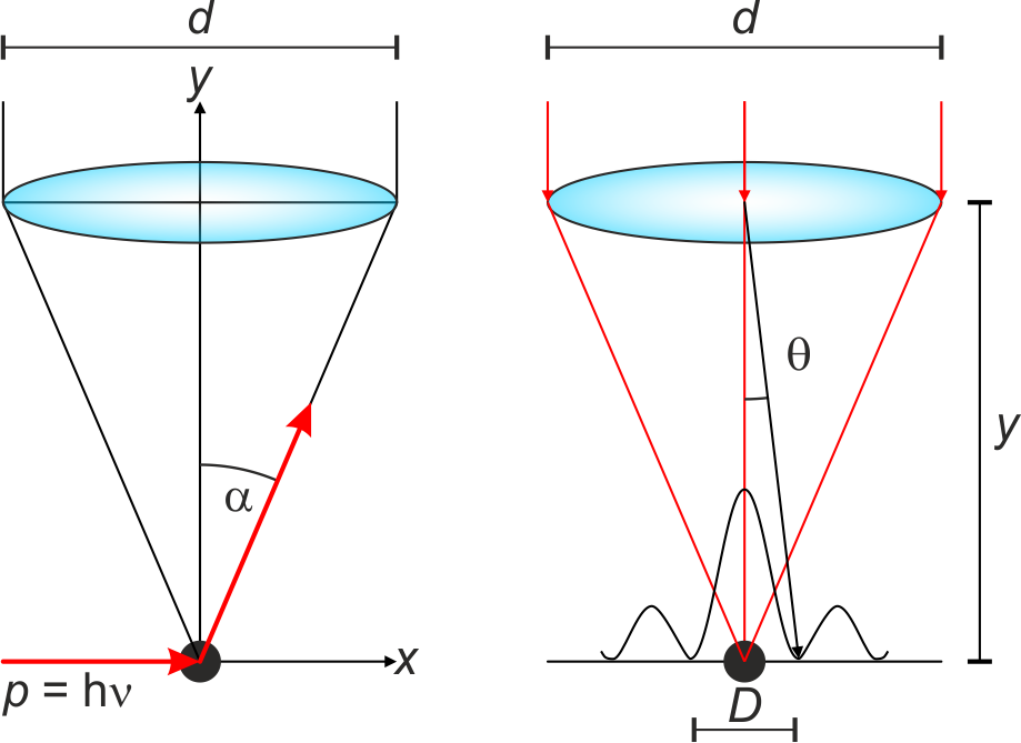
Another example might be constructed, if we assume to observe a microscopic particle at rest via a miocroscope.Therefore, we have to shine light on that particle in order to detect the scattered light of wavelength \(\lambda\) within the opening angle of the objective \(2 \alpha\) (\(\sin \left( \alpha\right) \approx \tan \left( \alpha\right) = d/\left( 2 y \right)\), with \(d\) and \(y\) being the diameter of the objective and the particle-objective distance, respectively). The momentum of the scattered photon then has an uncertainty along \(x\)

\[\Delta p_x = p_{\mathrm{ph}} \cdot \sin \left( \alpha \right) \approx \frac{h}{\lambda} \cdot \frac{d}{2 y}\]

Due to the conservation of overall momentum, the particle that scattered the photon (and got a momentum because of this event) has the same uncertainty \(\Delta p_x\). In addition, if parallel light is focused by means of an objective, diffraction at teh objective’s edge will lead to a diffraction pattern in teh focal plane. The central intensity maximum (0-th order diffraction peak) has a diameter of

\[1.22 = \frac{d}{\lambda} \,\sin \left( \theta \right) \approx \frac{d}{\lambda} \,\tan \left( \theta \right) = \frac{d}{\lambda} \frac{D}{2y} \mathrm{.}\]

Remember the lecture about diffraction and the Airy disk. As a consequence, we cannot determine the position of the particle more precise than \(\Delta x = D\) (the diameter of the Airy disk). If we now combine both equations, we get

\[= 1.22 \cdot h \mathrm{.}\]

Fig.: (left) A photon is scattered by a particle and propagtes within the opening angle of the objective. (right) In order to localize the particle, it has to be bigger than the Airy disc.

As we have learned on the basis of diffraction at a pinhole, one might use light with a shorter wavelength in order to reduce \(\Delta x\). However, at the very same moment one will increase \(\Delta p_x\) about the same amount one has decreased \(\Delta x\) resulting in a constant product \(\Delta x \cdot \Delta p_x\).

Energy-time uncertainty

As we have seen, the spatial distribution of the wave packet \(\Delta x\) depends on the wavenumber interval \(\Delta k\), used to construct the wave packet. Now we want to discuss how precise we can measure the energy \(\hbar \omega_0\) of a wave packet with the central frequency \(\omega_0\) if we measure during a time interval \(\Delta t\).

As we did previously, we comprise the wave packet as superpostion of partial waves, but do not integrate over the wavenumber interval \(\Delta k\) but rather over the frequency interval \(\Delta \omega\),

\[\psi \left( z,t \right) = \int_{-\infty}^{+\infty} C \left( \omega \right) \, \mathrm{e}^{i\left(\omega t - k z \right)} \, \mathrm{d} \omega \mathrm{.}\]

Completely analogous as in the previous case of matter waves we make us of a Taylor series

\[k = k_0 + \left( \frac{\mathrm{d}k}{\mathrm{d} \omega} \right)_{\omega_0} \left( \omega - \omega_0 \right) + \ldots\]

and substitute \(u = t - \left( \mathrm{d}k / \mathrm{d} \omega \right)_{\omega_0} \cdot z\), which allows us to calculate

\[\psi \left( z,t \right) =2 C \left( \omega \right) \; \frac{\sin \left( \Delta \omega \cdot u \right)}{u} \; \mathrm{e}^{i\left(\omega_0 t - k_0 z \right)} \mathrm{.}\]

At the fixed position \(z_0\) the maximum appears at \(t_0 = \left( \mathrm{d}k / \mathrm{d} \omega \right)_{\omega_0} \cdot z_0\) and the two roots left and right of the central maximum are at poistion \(z_0\) at times

\[t_{1,2} = \left( \frac{\mathrm{d}k}{\mathrm{d} \omega} \right)_{\omega_0} \cdot z_0 \pm \frac{\pi}{\Delta \omega} \mathrm{,}\]

respectively. Thus, the central maximum needs the time \(\Delta t = 2 \pi / \Delta \omega\) to completely pass the position \(x_0\). Conversely, if we record a wave packet onlöy within the time interval \(\Delta t\), then we can estimate its central frequency only with an uncertainty \(\Delta \omega\).

For example we measure a monochromatic wave \(C_0 \cdot \mathrm{e}^{i\left(k z -\omega_0 t \right)}\) at position \(z = 0\) during the interval \(\Delta t\). The Fourier transform of the amplitude distribution of this wave train then reads as

\[C \left( \omega \right) = \int_{t=-\Delta/2}^{+\Delta/2} C_0 \mathrm{e}^{i\left(\omega - \omega_0 \right)t} \mathrm{d}t = C_0 \frac{\sin\left(\frac{\omega - \omega_0}{2} \cdot \Delta t\right)}{\frac{\omega - \omega_0}{2} \cdot \Delta t} \mathrm{.}\]

The central maximum has a width of \(\Delta \omega = 2 \pi / \Delta t\). Since the energy is connected with the frquency in accord to \(E = \hbar \omega\), we finally obtain

\[\Delta E \cdot \Delta \omega \ge h \mathrm{.}\]

If we use a Gaussian distribution of the amplitude instead of a constant, we will result in \(\Delta E \cdot \Delta \omega \ge \hbar\). However, if we observe a particle only during a limitted period of time \(\Delta t\), we can estimate its energy only with the certainty of \(\Delta E \ge h/\Delta t\).

Spreading of wave packets

As we have seen previously the center of a matter wave propagates with the group velocity \(v_{\mathrm{g}}\) which is tantamount to the velocity of a particle \(v_{\mathrm{p}} = p/m\). Since the initial momentum of the particle \(p\) allready bears a particular uncertainty \(\Delta p\), we cannot determine the momentum of the particle more precise than \(p \pm \Delta p\). As a consequence \(v_{\mathrm{g}}\) also bears a particular uncertainty $ \Delta `v_{:nbsphinx-math:mathrm{g}`}$ with

\[\Delta v_{\mathrm{g}} = \frac{1}{m} \Delta p = \frac{1}{m} \frac{\hbar}{\Delta z_0} \mathrm{,}\]

with \(\Delta z_0\) being the uncertainty of the particle’s position at time \(t = 0\). Due to the uncertainty of the particle propagation, the uncertainty to determine \(\Delta z\) at a later time than \(t = 0\) grows with increasing time, namely

\[\Delta z \left( t \right) = \Delta v_{\mathrm{g}} \cdot t = \frac{\hbar}{m \Delta z_0} \cdot t \mathrm{.}\]

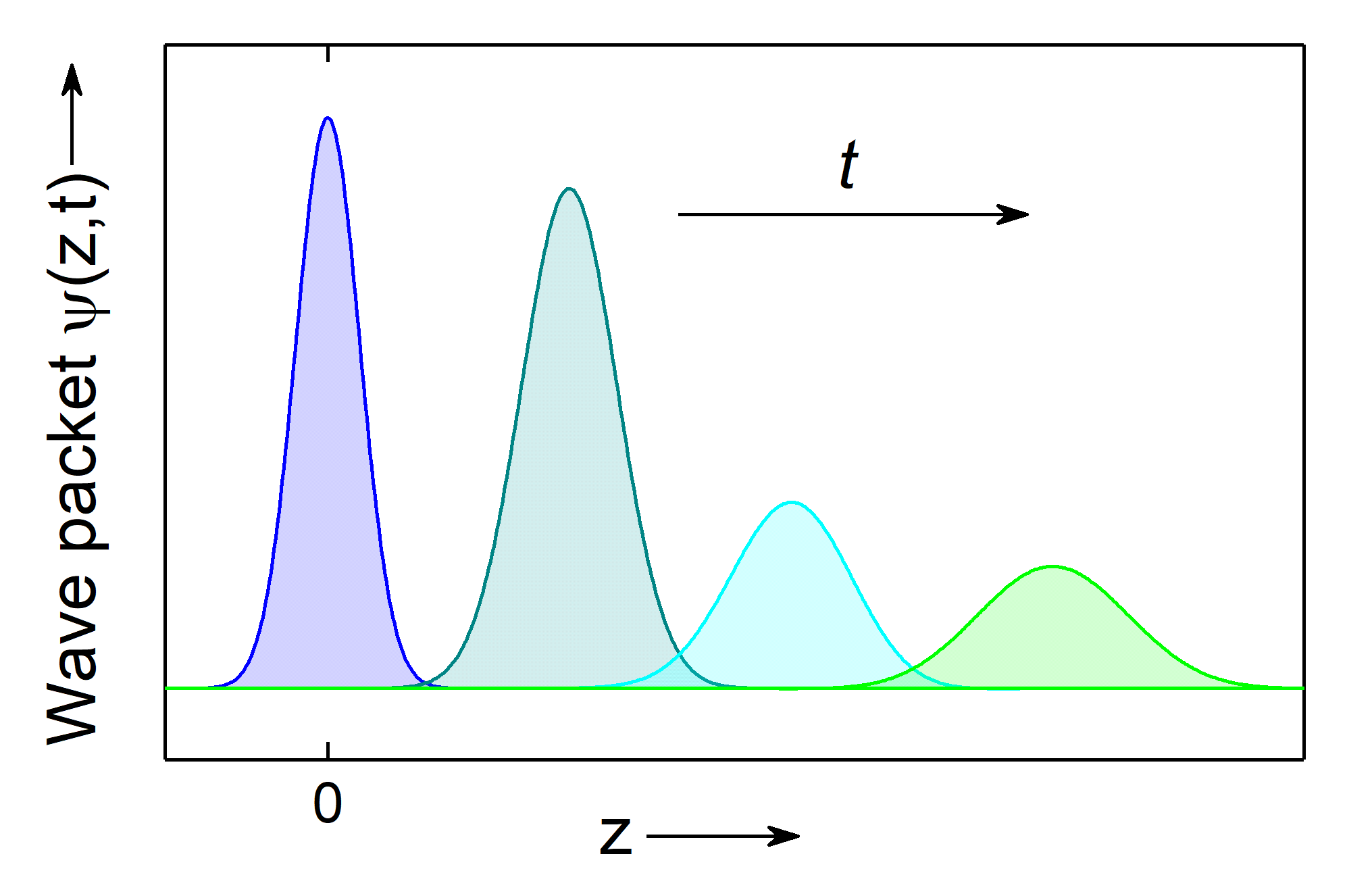
Here, \(\Delta z \left( t \right)\) denotes the width of the wave packet at time \(t > 0\). The area under the curve of the wave packet, however, remains constant. This is an immediate consequence of the normalization condiziont,

\[\int_{-\infty}^{+\infty} \left| \psi \left( z, t \right) \right|^2 \mathrm{d}z = 1 \mathrm{.}\]

Fig.: The spreading of a wave packet with Gaussian amplitude during time. Note the actual amplitude of the wave packet is decrasing while its width is increasing. The area under the curve, however, is constant.

Furthermore, it is evident that the better the particle is located at time \(t = 0\) (\(\Delta x_0\) small), the greater the spread over time. This arises from an increased momentum uncertainty as a consequence of the reduced position uncertainty, and hence an increased uncertainty of the particle velocity.